Rolling Down the Yield Curve
January 30, 2020 |

Disclaimer – The views and opinions expressed in this blog are those of the author and do not necessarily reflect the views of Scalable Capital Bank GmbH or its subsidiaries. Further information can be found at the end of this article.
This is the fourth post in our series on fixed-income securities. In the first blog posts we have seen how yield curves reflect the level of compensation that the financial market requires for lending money, how this level of compensation varies over timedepending on the prevailing market environment and how varying interest rates can be translated into varying fixed-income security prices. We now have a sound understanding of bond prices and their link to yield curves, but we still haven't yet addressed probably the most important question: what is an optimal investment strategy for fixed-income securities?
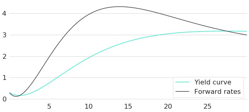
Obviously this heavily depends on the prevailing financial environment, expectations about future changes thereof, and an investor's risk preferences. In other words: a single optimum investment strategy for everyone does not exist. Still, let's try to answer this question with some arbitrarily chosen interest rate environment as a concrete example. The interest rate environment chosen can be seen in Figure 1 in terms of both yield curve and forward rates curve. So, given this environment: if we want to invest money for 1 year, bonds of which maturity should we buy?
We already know: bond prices will react to yield curve changes. Hence, an optimal investment will always depend on our expectations regarding how yield curves will change over time. For this scenario, let's first introduce two of the most popular theories on yield curves. Both could be an explanation for the observed upward sloping yield curve in our example.
Liquidity premium hypothesis: upward sloping yield curves are not an indication for rising spot rates in the future, but they are a result of people demanding some additional compensation when committing to lend money over multiple years. This way, upward sloping yields are not in contradiction with constant yield curves over time.
Expectation hypothesis: current forward rates are an unbiased estimator of future interest rates. In other words: today's forward rate between 9 and 10 years maturity is equal to the one year spot rate that will actually prevail 9 years in the future. This would imply that yield curves continuously change as forward rate curves are simply shifted to the left with passage of time.
Note: our definitions here are only capturing the main essence of both theories which are actually a bit more comprehensive. For example, the presence of liquidity premia is not automatically equivalent with constant yield curves over time. But for the sake of simplicity we will proceed with these rather intuitive definitions for now, such that the assumption of constant interest rates will be labeled as the liquidity premium hypothesis, and the expectation hypothesis represents the case where forward rates are perfect predictors for future spot rates.
Let's now say that we hold a zero-coupon bond with 10 years maturity for one year. Which compounding will we get under each of the two interest rate scenarios? The present value of this bond will be determined by the value of the yield curve at maturity equal to 10 years. And after one year, the new value of the bond will be given by the yield at maturity equal to 9 years. Since we are again working with yield curves under continuous compounding, another way of looking at the value of a bond is to determine the overall value of compounding by taking the integral of currently prevailing forward rates from 0 to maturity :
Hence, assuming that liquidity premia explain the upward slope of yield curves and that yield curves remain constant over time, the difference between the value of the bond today and next year will be the integral of the forward rate curve from 9 years to 10 years. Given that the expectation hypothesis holds, however, the difference in forward rate integrals will be completely different. Again, next year we will take the integral over 9 years only, as this will be the correct new maturity. However, forward rates will simultaneously shift to the left by one year, so that the new bond yield will effectively be given by the integral from maturity 1 to 10 over today's forward rate curve. Hence, the difference between today's yield and the yield in one year is just the integral of forward rates from 0 to 1 year. The relevant areas under the forward rates curve for both scenarios are shown in Figure 2.
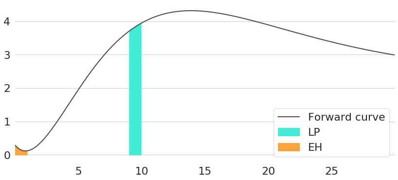
To conclude, the effective level of compounding during the next year will be completely different for both scenarios. With constant yield curves over time, compounding will be given by the integral over forward rates at the right end. In contrast, the integral on the left end will be relevant given that the expectation hypothesis holds. Note: in this case the actual maturity of the bond does not matter, and bonds of all maturities will have the exact same compounding during the first year.
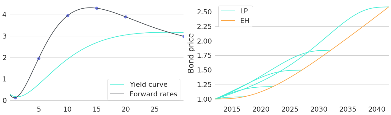
To further emphasise this point, let's now take a look at the price trajectories of 6 bonds of different maturities. The chosen maturities are highlighted by blue dots on the forward rate curve in the left subplot of Figure 3. The right chart shows their respective price trajectories: for the case of constant yields trajectories are plotted in turquoise, orange lines represent trajectories under the expectation hypothesis.
Again, we can see: given that the expectation hypothesis holds, bonds of all maturities will have equal compounding in simultaneous periods. All price trajectories lie on the same orange line and only end at different maturities. For the case of constant yields, however, price trajectories depend on the level of forward rates at the respective maturity. Forward rates are highest for bonds with 15 years maturity, so their price trajectories will show the highest slope of all bonds at the beginning.
Now let’s imagine the world would behave well enough such that yield curves really would remain constant over time. From the last section we know that the compounding we harvest is proportional to the area under the forward rate curve at the respective maturity. Hence, in order to maximise compounding, we just need to find the maturity with maximum forward rates. One problem, however, is that the maturity that we hold actually changes continuously since it shortens with passage of time. Without rebalancing a maturity of 10 years today will only be a maturity of 7 years when held 3 years into the future from now. Hence, in order to always occupy the sweet spot of the yield curve we would need to continuously rebalance. This is called "rolling" fixed-income securities. In a world with transaction costs, the optimisation problem would boil down to finding an optimal tradeoff between rolling costs and targeting the optimal maturity range.
In reality, however, yield curves are far from constant over time. Still, rolling long-term fixed-income securities actually can be a good way to maximise expected returns (in the long run). However, there is no such thing as a free lunch and risks are the currency that needs to be paid for returns. Rolling over fixed-income securities of long maturities hence not only comes with higher returns, but also with higher risks. We will analyse this in further detail in the next blog posts in this series.
Disclaimer – The views and opinions expressed in this blog are those of the author and do not necessarily reflect the views of Scalable Capital Bank GmbH, its subsidiaries or its employees ("Scalable Capital", "we"). The content is provided to you solely for informational purposes and does not constitute, and should not be construed as, an offer or a solicitation of an offer, advice or recommendation to purchase any securities or other financial instruments. Any representation is for illustrative purposes only and is not representative of any Scalable Capital product or investment strategy. The academic concepts set forth herein are derived from sources believed by the author and Scalable Capital to be reliable and have no connection with the financial services offered by Scalable Capital. Past performance and forward-looking statements are not reliable indicators of future performance. The return may rise or fall as a result of currency fluctuations. Please refer to our risk information.
Risk Disclaimer – There are risks associated with investing. The value of your investment may fall or rise. Losses of the capital invested may occur. Past performance, simulations or forecasts are not a reliable indicator of future performance. We do not provide investment, legal and/or tax advice. Should this website contain information on the capital market, financial instruments and/or other topics relevant to investment, this information is intended solely as a general explanation of the investment services provided by companies in our group. Please also read our risk information and terms of use.