Yield Curves: Common Patterns in Prices of Fixed-Income Securities
29. Oktober 2019 |
Disclaimer – The views and opinions expressed in this blog are those of the author and do not necessarily reflect the views of Scalable Capital Bank GmbH or its subsidiaries. Further information can be found at the end of this article.
Whenever we deposit money at a bank account, this means that we effectively lend money to the bank. The bank will take most of the deposit and try to earn some money with it by investing it in the financial markets or lending it out as loans. As the bank expects to earn money with it, it usually is also willing to pay some compensation to us, which is generally quoted in terms of interest rates. Aside from lending money to a bank through deposits, the compensation that we get for lending in the financial markets is not usually quoted in terms of interest rates. Instead, fixed-income securities just define a series of future cash-flows at future points in time. Lending money to a company or government simply means buying the entitlement to a series of these cash-flows, and depending on the price that we pay for this entitlement, we will either get higher or lower compensation for lending the money. Given that many fixed-income instruments are actively traded in secondary markets, we usually have a representative price for a lot of fixed-income instruments. When prices, size, and dates of all future cash-flows are known, one can infer an estimate for the implicitly given level of compensation, e.g. by computing the internal rate of return (i.e. the yield of the security). By doing this one usually finds that bonds of roughly similar maturity tend to have similar rates of return. In other words, there is some hidden structure in the prices of fixed-income securities.
The most popular way of representing this common underlying structure is by estimating a relationship between maturity and compensation, a so-called yield curve. For each maturity it determines the annualised interest rate that is used by the market to discount a future cash-flow. However, annualised interest rates given by a yield curve cannot be directly observed in financial markets. They are estimated values that are inferred from fixed-income prices through the help of assumptions that determine how smoothly interest rates should change for varying maturities. Two of the most popular methodologies for this are the Svensson yield curve model (Svensson 1994) or a model based on a quasi-cubic hermite spline function which is for example used by the US Treasury1. Given the structural assumptions that are implicitly defined by the yield curve model that is used, any given estimated yield curve will never fully match all fixed-income prices perfectly. Variable parameters of a yield curve model are determined such that derived fixed-income prices match observed market prices as closely as possible. This, however, is only meaningful if fixed-income securities have roughly similar characteristics. Most importantly, they should be aligned with regards to credit quality. As future cash-flows will only occur when the debtor is able to repay, all cash-flows do come with a (sometimes negligible) probability of default. For the US government (and other trusted developed market countries) this probability is usually assumed to be zero. But as soon as default probabilities are not perceived to be negligible, the market requires some additional compensation for the credit risk that is inherent. This compensation will lead to market prices trading below those of comparable risk-free securities, like with corporate bonds or emerging market government bonds. This way two bonds with equal future cash-flows, but differing credit quality, would be traded at different market prices. Hence, it does not make sense to estimate yield curves for a group of bonds with different credit quality, because it would be impossible to match all prices reasonably closely. Yield curves will generally be estimated for buckets of similar credit quality, such that each credit quality gets its own yield curve.
Given that we have an estimate for a yield curve, we can now compute the present value for any future cash-flow. However, one additional piece of information is necessary: the unit of measurement of interest rates so to speak. Interest rates quantify the magnitude of compounding, but the actual frequency of compounding also needs to be defined. So any quoted interest rate could lead to different aggregate compounding depending on whether interest payments occur once per year (annually), twice per year (bi-annually) or even infinitesimally frequently (continuous compounding). While annual and bi-annual compounding actually might occur in reality for bank accounts, you will usually never encounter continuous compounding in real life. However, stating yields in terms of this unit of measurement happens quite frequently, because it allows for straightforward transformations and simple computations of present values for given interest rates. With given interest rates of 6% we will get the following different market prices for a cash-flow of 100 EUR with maturity of one year:
The information of yield curves can be expressed in three ways:
All three fundamentally represent the same information, but each of them through a different perspective.
Discount functions are a kind of inverse perspective on interest rates and compounding. Instead of telling you how much interest rates you get for a given amount of money that you invest today, discount functions give you an answer to the opposite direction: 1 EUR in the future is worth how much today? The nice thing about them is: there is only one unit of measurement, so they are uniquely defined. Yields and forward rates are somewhat auxiliary constructs to identify common patterns in fixed-income security prices and as such they depend on the unit of measurement (e.g. annual or bi-annual compounding). Discount functions, in contrast, can be directly observed in the form of market prices for some durations, and there is only one unit of measurement for market prices. However, the downside of discount functions is that they are not easily interpretable. Saying that the discount function for maturity 3 years has a value of 0.86 is much harder to interpret than saying that annualised interest rates for such a duration are 5%.
Forward rates express compounding of money during time intervals in the future. In forward rate curves, these time intervals become infinitesimally small, such that each point represents instantaneous compounding at some future point in time. This is not to say that this value will really materialise in the future, but it is the level of compounding that one could lock in today.
Yields express compounding of money for different durations when money is invested today. As such, the yield at time with maturity given by is the average of forward rates for the interval . Yields are normalised to some unit of measurement, however. In most cases they are annualised in order to make yields of different maturities better comparable.
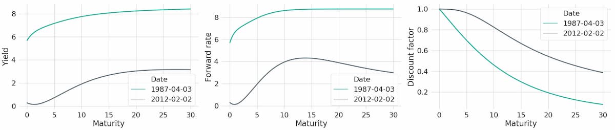
An example for how yield curves and matching forward rate curves and discount functions look like can be seen in Figure 1. In this chart, yields and forward rates are quoted in terms of continuous compounding. Using continuous compounding, there is a straightforward relationship between yields and forward rates. For any given duration, the yield is equal to the average of all forward rates from zero to that duration:
Although some formulae become particularly straightforward for yields that are quoted in terms of continuous compounding, it sometimes also comes with advantages to quote yields in different units of measurements, e.g. par yields. Most bonds with maturity above one year are usually coupon paying bonds and their coupon rates are defined in such a way that they trade almost at par at issuance. This means that coupon rates are determined such that the bonds' market prices will be almost equal to their notional in the beginning. For example, let's take a bond with notional 100 EUR, annual coupon payments of 4 EUR and maturity of 10 years. Over the full lifetime, such a bond will generate coupon payments of 40 EUR. Hence, given an overall value of future cash-flows of 140 EUR, a significant part of cash-flows will be obtained even prior to maturity. Yield curves are usually upward sloping, with higher yields for higher maturities. Hence, if continuously compounded interest rates with duration 10 years were equal to 4%, then all cash-flows before 10 years would usually be discounted with interest rates below 4%. Discounting with lower rates will increase the present value of future cash-flows, such that the coupon bearing bond would have to trade above par. Or, in turn, the yield at maturity 10 years would need to be larger than 4% if the bond was traded at par. Simply looking at coupon rates of newly issued bonds will not allow an easy translation to continuously compounded yields. So if a close connection between coupon rates and yields is desired, one should look at par yields instead.
In the first paragraph we mentioned two methods of how yield curves can be estimated from fixed-income security prices. Estimating yield curves is a non-trivial and cumbersome process. In the first step, one needs to define a basket of fixed-income securities that should be used as inputs for the estimation. In particular, the basket should only contain securities of comparable credit quality. Secondly, for each security one needs to consider all specified future cash-flows, both in terms of their magnitude as well as their exact timing. And finally, a given yield curve model needs to be estimated in such a way that security prices derived from the estimated yield curve match observed market prices as closely as possible. Luckily, we do not need to perform this estimation process ourselves for the most popular markets like US Treasuries or European government bonds, because we can safley rely on estimated interest rates from a number of public sources.
One such source is the dataset of estimated US Treasury yield curves provided by The Federal Reserve Board2. The dataset consists of daily parameter estimates of Svensson yield curve models applied to the US Treasuries from 1961 to the present. Yields are quoted in terms of continuous compounding, and yield curves are estimated by imposing the following functional form on forward rate curves (see Gurkaynak et al. 2006):
If we are only interested in how interest rates change over time for some popular maturities (e.g. 1 year or 10 years), the dataset is a bit cumbersome to deal with, because it only provides the parameters of the yield curves, but not the yields themselves. However, this has the additional benefit that we can evaluate yield curves at any arbitrary maturity and are not constrained to a subset of constant maturities. In particular, if we want to price fixed-income securities with arbitrary cash-flows as precisely as possible, we would otherwise have to interpolate between interest rates of constant maturities in order to perfectly match the maturities of all cash-flow dates. So once you already have the framework to translate yield curve parameters into yields, it is more informative to have the full yield curve available instead of having some constant maturities only.
In this blog post we have given a short introduction to yield curves and how they can be used to represent common patterns in fixed-income security prices. However, this is only the first blog post in a series on fixed-income securities and interest rates. In particular, we are going to examine in more detail how interest rate changes can affect the prices of fixed-income securities and bond ETFs. Furthermore, we will also take a look at historic data to get a feeling about the magnitude of interest rate risks that prevail when holding fixed-income securities. To set the stage for these empirical applications, Figure 2 shows the historic yield curves obtained from the Federal Reserve dataset that we mentioned above.
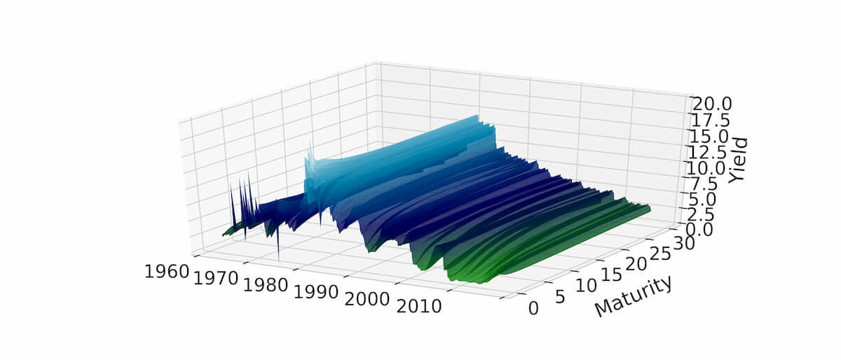
As can be seen from the chart, interest rates have varied wildly over the last 60 years, with interest rates ranging from roughly 15% in the 1980s to around 0% for short-term holding periods in 2018. Some of the extreme fluctuations at the very short end of the yield curve in the first half of the data sample are of artificial nature, however. Yield curves in this dataset have been fit to bond prices with maturity longer than 1 year only, such that any yield below 1 year has to be obtained by extrapolation. What these interest rate changes meant for prices of fixed-income securities, to what extent variations are driven by inflation, and whether interest rates are a good predictor for recessions - we will try to find answers to all of these questions in the next posts.
Svensson, L. E. O. (1994), Estimating and Interpreting Forward Rates: Sweden 1992-4, National Bureau of Economic Research Working Paper #4871.
Gurkaynak, Refet. S., Sack, Brian, and Wright, Jonathan H. (2006), The U.S. Treasury Yield Curve: 1961 to the Present, Federal Reserve Board Finance and Economics Discussion Series.
1: Cubic splines Treasury methodology: https://www.treasury.gov/resource-center/data-chart-center/interest-rates/Pages/yieldmethod.aspx
2: The U.S. Treasury Yield Curve of The Federal Reserve Board: https://www.federalreserve.gov/pubs/feds/2006/200628/200628abs.html. The same dataset can also be accessed more conveniently through Quandl: https://www.quandl.com/data/FED/PARAMS
Disclaimer – The views and opinions expressed in this blog are those of the author and do not necessarily reflect the views of Scalable Capital Bank GmbH, its subsidiaries or its employees ("Scalable Capital", "we"). The content is provided to you solely for informational purposes and does not constitute, and should not be construed as, an offer or a solicitation of an offer, advice or recommendation to purchase any securities or other financial instruments. Any representation is for illustrative purposes only and is not representative of any Scalable Capital product or investment strategy. The academic concepts set forth herein are derived from sources believed by the author and Scalable Capital to be reliable and have no connection with the financial services offered by Scalable Capital. Past performance and forward-looking statements are not reliable indicators of future performance. The return may rise or fall as a result of currency fluctuations. Please refer to our risk information.
Risikohinweis – Die Kapitalanlage ist mit Risiken verbunden und kann zum Verlust des eingesetzten Vermögens führen. Weder vergangene Wertentwicklungen noch Prognosen haben eine verlässliche Aussagekraft über zukünftige Wertentwicklungen. Wir erbringen keine Anlage-, Rechts- und/oder Steuerberatung. Sollte diese Website Informationen über den Kapitalmarkt, Finanzinstrumente und/oder sonstige für die Kapitalanlage relevante Themen enthalten, so dienen diese Informationen ausschließlich der allgemeinen Erläuterung der von Unternehmen unserer Unternehmensgruppe erbrachten Wertpapierdienstleistungen. Bitte lesen Sie auch unsere Risikohinweise und Nutzungsbedingungen.