Impacts of Yield Curve Changes on Fixed-Income Security Prices
7. Januar 2020 |
Disclaimer – The views and opinions expressed in this blog are those of the author and do not necessarily reflect the views of Scalable Capital Bank GmbH or its subsidiaries. Further information can be found at the end of this article.
This is the third post in our series on fixed-income securities. In the first two blog posts we have seen how yield curves reflect the level of compensation that the financial market requires for lending money, and how this level of compensation varies over time depending on the prevailing market environment. In this part we will examine how varying interest rates can be translated into varying fixed-income security prices.
For pricing, any fixed-income security can be treated as a set of cash-flows that occur at future points in time. These future cash-flows can then be translated to present values using discount factors :
For the special case of zero-coupon bonds (i.e. bonds with a single future payment only) with nominal value of 1 EUR, bond prices coincide with discount rate curves. Given some arbitrarily chosen yield curve from 1987, the associated discount rate function lets one easily read off bond prices for zero-coupon bonds of each maturity. This can be seen in Figure 1. The red dot in the left subplot exemplarily shows the price of a zero-coupon bond with a maturity of 5 years. Similarly, we could find a price for zero-coupon bonds of each maturity.
Given that we only know today's yield curve, we do not know future zero-coupon bond prices yet. To get the next day's price we would need to adapt the maturity of the bond (which is now one day less), and evaluate tomorrow's discount function at this maturity. However, to get a first feeling on how bond prices could evolve over time, we will artificially hold the yield curve constant over the subsequent years as shown in the subplot in the middle of Figure 1. Now we can easily compute future bond prices by evaluating the same discount function at continuously decreasing maturities. This bond price evolution can be seen in the subplot on the right. It basically shows the same line (though only part of it) that we also could see in the leftmost chart on the lefthand side of the red circle, but from right to left (i.e. horizontally flipped).
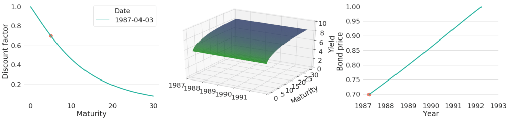
Figure 1: Discount Factor and Price Evolution of a Zero-Coupon Bond with Constant Yield Curves
Zero-coupon bonds only have a single payment: the notional at maturity. Hence, when yields remain constant, bond prices can only increase over time (given that interest rates are not negative) to reflect compounding. This will look differently for coupon bonds, where cash-flows also occur during the lifetime of the bond. Any coupon payment needs to be reflected in bond price drops of equal amount - otherwise it would be worthwhile to buy the bond one day before coupon payment and immediately sell it afterwards again just to collect the coupon payment. For the constant yield curve shown on the left in Figure 2, the right subplot shows associated bond price trajectories for both a zero-coupon bond as well as a coupon paying bond. The coupon-paying bond has semi-annual payments with coupon rate 7%, so that it will pay 3.5 EUR every six months. Hence, bond prices will regularly drop by 3.5 EUR and in between they rise due to compounding.
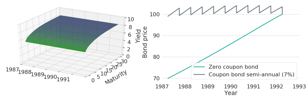
Figure 2: Price Evolutions of a Zero-Coupon and a Coupon Bearing Bond with Constant Yield Curves
Of course, in reality yield curves will not be constant over time (see our previous blog article) and any change of yield curves in turn will have an effect on the discounting of future cash-flows and will thereby change the prices of bonds. To see this effect, let's now artificially insert a rather dramatic change in yields in the middle of the period: yields now suddenly drop as shown in the left part of Figure 3. Decreasing yields will lead to decreased discounting, such that future cash-flows will become of greater value when measured in terms of today's price level. This will hence increase bond prices. The effect can be seen in the right chart of Figure 3.
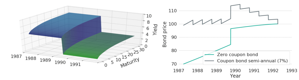
Figure 3: Price Evolutions of a Zero-Coupon and a Coupon Bearing Bond when there is a Single Yield Curve Shift
Let's now look at a more realistic scenario: yields are neither constant over time, nor will they change as dramatically as in the previous example. Figure 4 shows prices for the same two bonds, but this time using the true historic yield curve evolution of US Treasury yields.
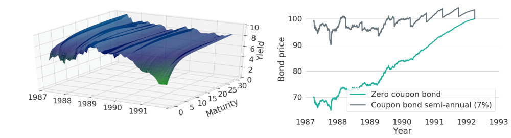
Figure 4: Price Evolutions of a Zero-Coupon and a Coupon Bearing Bond for Continuously Varying Yield Curves
We have already seen that decreasing (increasing) yields will lead to increasing (decreasing) bond prices. But does this really show the full picture? What we have left unconsidered so far in all the examples above is the fact that intermediate cash-flows could be re-invested. Let's say a coupon bond has maturity of June 1st, 2010, a notional of 100 EUR and a coupon payment of 1.75 EUR at June 2nd, 2008. Then at the day of the coupon payment the amount could be re-invested again until the final maturity of the bond (and potentially even beyond). Hence, 1.75 EUR can be invested into a zero-coupon bond from 2008 to 2010 (assuming that a matching zero-coupon bond exists in the bond market). Depending on the yield curve prevailing at the time of re-investment, the 1.75 EUR might increase in value until maturity. Doing an exact calculation for all obtained coupon payments, one could keep track of the aggregate value of accrued re-investments at each point in time. Figure 5 shows an exemplary computation of total return bond values.
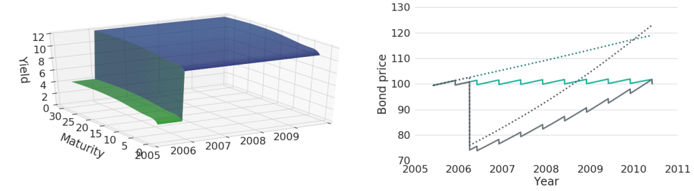
Figure 5: Bond Price and Total Return Evolutions for Constant Yields and Upwards Shifted Yields
On the left side of the chart we can see a constructed yield curve scenario with a single increase of interest rates. On the right, we can see the associated trajectories of bond prices and total return values in grey. The dotted grey line represents the total return values with re-investment of coupon payments. In contrast to the solid grey line, it does not have the regular downwards shifts caused by coupon payments, because coupon payments are immediately re-invested and hence the money will not leave the asset position. Still, both grey series experience a huge price decline in 2006 that is caused by the interest rate shock that we simulated. Due to this huge price decline, one might be inclined to think that the interest rate shock did have a negative overall effect on both price series. However, if we compare the price series to the respective price series that we would get under a scenario of constant interest rates (shown in turquoise), one can see that the upwards shift of interest rates actually leads to a better total return outcome than what we would get with constant interest rates. The bond price series themselves end in the same point, because independent of the interest rate scenario one will receive the notional at maturity. However, when coupon payments can be re-invested, any re-investment can be done at a higher interest rate level after the interest rate shift, such that the total return actually increases. The opposite effect will happen for the case of a sudden decrease in yields: bond prices will suddenly jump upwards, but any coupon payments will have to be re-invested at lower rates. Ultimately, this will decrease total returns. Note, however, that the approach so far makes one important assumption for simplicity: coupon payments will always be re-invested exactly to maturity of the original coupon bond. In reality, however, there is no reason why coupon payments should not be re-invested with arbitrary maturity.
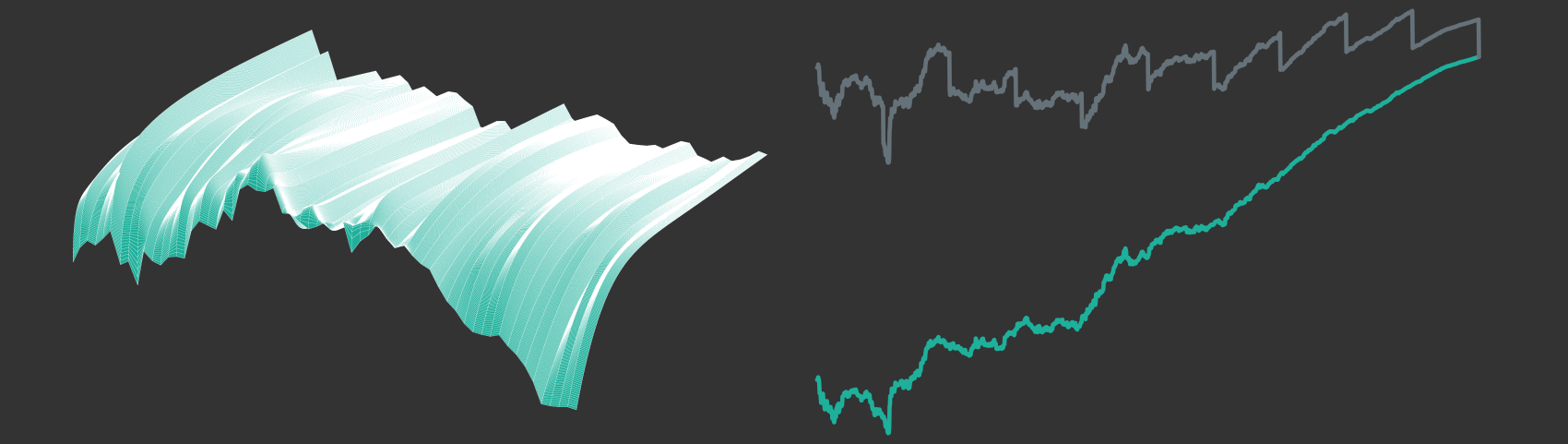
Let's now look at total returns for an example of real historic US Treasury yield curves. Figure 6 shows trajectories of historic yield curves on the left side, while bond prices and bond total return values are shown on the right. Grey lines again show the prices with regards to the interest rates shown on the left, while turquoise lines represent prices under constant yield curves for comparison. As can be seen from the chart, although historic yield curves did vary quite significantly over time, total returns are pretty similar to the case of constant yields in this selected time period. Non-linear interactions between yield curve changes, bond prices and re-investments of coupon payments make the effect of continuous yield curve changes on total returns very hard to predict.
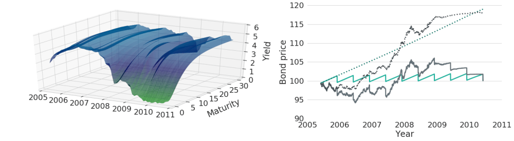
Figure 6: Bond Price and Total Return Evolutions for Constant Yields and Continuously Varying Historic Yields
Disclaimer – The views and opinions expressed in this blog are those of the author and do not necessarily reflect the views of Scalable Capital Bank GmbH, its subsidiaries or its employees ("Scalable Capital", "we"). The content is provided to you solely for informational purposes and does not constitute, and should not be construed as, an offer or a solicitation of an offer, advice or recommendation to purchase any securities or other financial instruments. Any representation is for illustrative purposes only and is not representative of any Scalable Capital product or investment strategy. The academic concepts set forth herein are derived from sources believed by the author and Scalable Capital to be reliable and have no connection with the financial services offered by Scalable Capital. Past performance and forward-looking statements are not reliable indicators of future performance. The return may rise or fall as a result of currency fluctuations. Please refer to our risk information.
Risikohinweis – Die Kapitalanlage ist mit Risiken verbunden und kann zum Verlust des eingesetzten Vermögens führen. Weder vergangene Wertentwicklungen noch Prognosen haben eine verlässliche Aussagekraft über zukünftige Wertentwicklungen. Wir erbringen keine Anlage-, Rechts- und/oder Steuerberatung. Sollte diese Website Informationen über den Kapitalmarkt, Finanzinstrumente und/oder sonstige für die Kapitalanlage relevante Themen enthalten, so dienen diese Informationen ausschließlich der allgemeinen Erläuterung der von Unternehmen unserer Unternehmensgruppe erbrachten Wertpapierdienstleistungen. Bitte lesen Sie auch unsere Risikohinweise und Nutzungsbedingungen.