Yield Curve Empirics
December 4, 2019 |
Disclaimer – The views and opinions expressed in this blog are those of the author and do not necessarily reflect the views of Scalable Capital Bank GmbH or its subsidiaries. Further information can be found at the end of this article.
In the first blog post of this series on fixed-income securities we have seen how yield curves reflect the level of compensation that the financial market requires for lending money. This level of compensation is derived from market prices of fixed-income securities and as such it significantly varies over time depending on the prevailing market environment. How this level of compensation did vary in the past is the subject of this blog post, which explores historic yield curves for multiple markets.
The whole analysis of this post can be done with publicly available data, as most central banks provide historic data on several interest rates. However, interest rates of different central banks generally do not come with a fully aligned setup. In particular, interest rates could differ with regards to the methodology used to compute them, their unit of measurement or the selection of eligible securities that are used for estimation. For example, interest rates could be given as zero-coupon yields with continuous compounding, as par yields with bi-annual compounding, or one of multiple other different units. Knowing this unit of measurement is particularly important if the data is used for pricing of fixed-income securities, because the unit will determine the exact formula that is required to translate yield curves back to security prices. Hence, we will also give some background on all data shown, such that it becomes more clear how to use it in potential applications.
Let's start with interest rates estimated from US Treasury securities. Probably the easiest way to get US interest rate data is by downloading constant maturity Treasury (CMT) rates from the US Treasury. Constant maturity means that on each date the respective estimated yield curve is evaluated at certain constant maturities. This way, fixed-income security prices are used to determine the parameters of a yield curve, such that interest rates can also be estimated for maturities where no matching fixed-income security is available. This data can also be obtained from Quandl. Please note the following characteristics of these CMT rates which can also be found on either the Treasury Yield Curve Methodology page or the Frequently Asked Questions page:
„Negative Yields and Nominal Constant Maturity Treasury Series Rates (CMTs): At times, financial market conditions, in conjunction with extraordinary low levels of interest rates, may result in negative yields for some Treasury securities trading in the secondary market. Negative yields for Treasury securities most often reflect highly technical factors in Treasury markets related to the cash and repurchase agreement markets, and are at times unrelated to the time value of money.
At such times, Treasury will restrict the use of negative input yields for securities used in deriving interest rates for the Treasury nominal Constant Maturity Treasury series (CMTs). Any CMT input points with negative yields will be reset to zero percent prior to use as inputs in the CMT derivation. This decision is consistent with Treasury not accepting negative yields in Treasury nominal security auctions.
In addition, given that CMTs are used in many statutorily and regulatory determined loan and credit programs as well as for setting interest rates on non-marketable government securities, establishing a floor of zero more accurately reflects borrowing costs related to various programs.“
Now that we know the data that we are dealing with, let's take a look at it. Figure 1 shows CMT rates over time since January 1st, 1990 for several maturities: four different maturities below one year and eight maturities of at least one year. As we can see, there was a rather persistent downward trend of interest rates, particularly for rates of longer durations. In line with what we have read regarding negative yields there is not a single observation for any maturity that is below zero, even though interest rates have been fairly close to zero at the short end for a period of multiple years between 2008 and 2016. Only afterwards have they increased again such that rates of all maturities are between 1.5% and 2.5% at the time of writing.
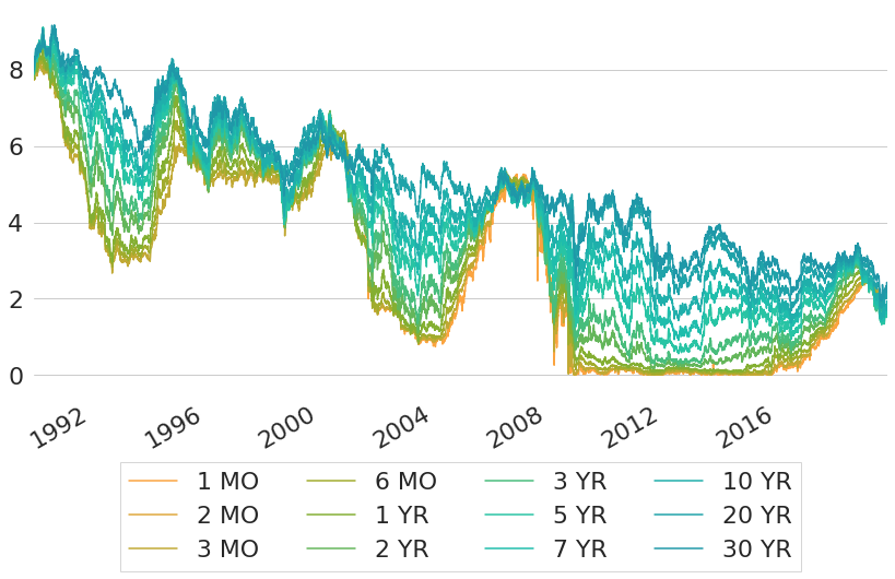
Figure 1: Historic Constant Maturity US Treasury Rates
Although the CMT rates dataset can be used quite conveniently to get an overview of interest rates over time, my preferred dataset for US Treasury yields is the one published by the Federal Reserve where yields follow the methodology of Gurkaynak et al. 2006. This dataset consists of daily parameter estimates of a Svensson yield curve model (Svensson 1994) with continuous compounding applied to US Treasuries from 1961 to the present. It also can be obtained from Quandl. Given the parameters over time, one can derive a yield curve for each day given the functional form of the Svensson yield curve model. This functional form can be expressed in terms of either yields, forward rates or discount functions, but it is most concisely expressed for forward rates:
In Figure 2 we can see yields over time that we get by converting forward curves into yield curves and evaluating these yield curves at constant maturities over time. From this chart we can see that the downwards trend of interest rates actually already persists since the 1980s, where rates of all maturities have been above 12%. And before that time, the evolution of interest rates has been characterised by an upward trend that pushed interest rates from a range of 2.5% to 5% for all maturities at the beginning of the dataset to above 12% within 15 years. From the chart we can also see that the level of interest rates that we face today is pretty similar to the level of rates that prevailed at the beginning of the dataset. Probably unexpectedly at that time, the period of low interest rates in the 1960s was followed by a period of astonishingly high interest rates in the 1980s. This raises the question: should we expect interest rates to rise again to such heights at some point in the future, if such an increase already happened in the past? Or what are driving forces behind interest rates that might have changed and will lead to a different behaviour of interest rates going forward?
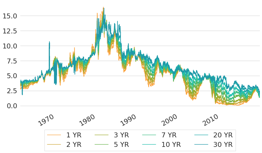
Figure 2: Historic Constant Maturity US Treasury Rates from Svensson Yield Curves
But before we try to find an answer to these questions, there is one misleading characteristic of the chart that deserves mentioning. From the chart it seems like long-term interest rates would experience sudden temporary shifts from time to time. For example, long-term rates jumped from roughly 5% to 10% and back again in a very short time in 1970. However, this is just an artefact of the data which is caused by the selection of fixed-income securities that are used to estimate the yield curve parameters. In this particular case, the problem is that 30 year Treasury securities did not exist at that time. Hence, interest rates for such long maturities have to be estimated with market prices of fixed-income securities of shorter duration only. In other words: the estimated yield curve has to extrapolate, going beyond the range of maturities where market prices actually exist. This might not work too well some of the time. A similar distortion also exists on the short end of interest rates, as this part of the yield curve is estimated from bond prices with maturity longer than 1 year, such that any yield below 1 year has to be obtained by extrapolation. So one important takeaway is that one should always be aware of the set of underlying securities that were used for estimation, because for any interest rates for maturities outside of this set the yield curve might not be particularly representative.
As we have seen so far, US interest rates have varied wildly over the last 50 years. Hence, the question arises: what exactly were the driving forces behind these large fluctuations of interest rates? Probably the most important force behind these changes is the Effective Federal Funds Rate which represents the weighted average of rates at which financial institutions trade federal funds. Federal funds are reserves held at the Federal Reserve Banks. Institutions with excess liquidity lend money overnight to other banks that are in need of further liquidity. Although the rate that needs to be paid from the borrowing institution is freely negotiated between both counterparties, it is strongly influenced by the Federal Reserve through open market operations or by buying and selling government bonds. This way, the Federal Reserve tries to navigate the Effective Federal Funds Rate into a direction such that it is in line with the Federal Funds target rate that was determined in the previous Federal Open Market Committee (FOMC) meeting. The Effective Federal Funds Rate is the most important interest rate in the US financial markets and it influences all other interest rates. Figure 3 shows the Effective Federal Funds Rate from the FRED Economic Data section2 of the Federal Reserve Bank of St. Louis together with two different constant maturity rates. As can be seen, constant maturity rates of 1 year maturity almost perfectly move in line with the Effective Federal Funds Rate. But even 10 year CMT rates follow the Effective Federal Funds Rate to a significant degree.
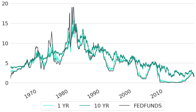
Figure 3: Historic Constant Maturity US Treasury Rates Compared to Federal Funds Rate
So if the Effective Federal Funds Rate has such a huge influence on short-term yields, the question arises: how does the FOMC actually determine which level of rates to target? Since the late 1970s, the Federal Reserve System and the FOMC have been instructed with the so-called "dual mandate": interest rates should be set in such a way that they effectively promote the goals of both maximum employment and price stability3. So in order to make its monetary policy decisions, the FOMC needs to have a good understanding of how interest rates interact with inflation and the economy. On a higher level, these quite complicated relationships are described by FRED as follows2:
„If the FOMC believes the economy is growing too fast and inflation pressures are inconsistent with the dual mandate of the Federal Reserve, the Committee may set a higher federal funds rate target to temper economic activity. In the opposing scenario, the FOMC may set a lower federal funds rate target to spur greater economic activity.“
Given the dual mandate of the FED, inflation is already set to have an impact on interest rate decisions by specification. This relationship we now want to see with data as well. As a measure of inflation we will use Consumer Price Index (CPI) data measured by the US Bureau of Labor Statistics. CPI data measures the average prices paid by urban consumers for a basket of goods and services. In particular, we will use core CPI data4 to derive inflation rates, such that food and energy prices are excluded from the basket, because both tend to have comparatively volatile prices. For more details on CPI data you can also have a look at the CPI FAQ page. Changes of core CPI over time can be seen in Figure 4, in comparison to the 1 year and 10 year CMT rates. As we can see, there is a similar downwards trend in inflation rates to the downwards trend that we have seen for interest rates. During the 1980s, inflation rates reached levels above 10% in some years. After that, inflation rates gradually decreased to a level of roughly 2% in recent years.
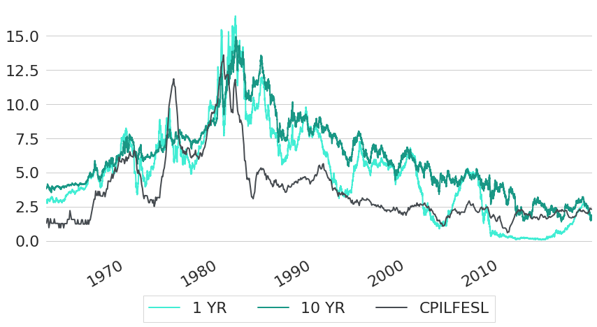
Figure 4: Historic Constant Maturity US Treasury Rates Compared to Inflation Rates
Note: General wisdom seems to be that inflation rates and interest rates are negatively correlated. An increase in interest rates will decrease the supply of money, and hence the value of money will increase (so inflation decreases). But from Figure 4 we can see that inflation rates and yields actually do have a rather positive relationship. A different way to also see this is by looking at inflation rates and interest rates in the cross-section of individual countries, like it is shown in Figure 5 for two exemplary years: 2005 and 2018. The data used for the charts is similar to Uribe 2018: CPI inflation rates5 and interest rates derived from lending rates6 and risk premia on lending7 from the World Development Indicators database provided by The World Bank.
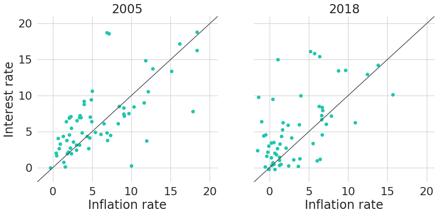
Figure 5: Inflation Rates and Interest Rates for Selected Countries
It actually makes sense that interest rates and inflation rates are rather positively related in the long run, because the difference between both is another meaningful financial indicator: the real rate. It measures the compensation for lending money at financial markets after subtraction of inflation rates. Only when interest rates and inflation rates move approximately in line (hence having a positive relationship) it is ensured that real rates also stay within a reasonable range. One potential way to compute real rates is by subtracting the inflation rates that we get from core CPI from CMT rates as shown in Figure 6. But keep in mind that this is just a rough proxy for real rates due to mainly two reasons. First, prevailing interest rates are actually forward looking, while inflation rates are backwards looking: CPI measures the evolution of prices in the past. And second, we did not correct for differences in maturities. The real rates shown are just the difference between interest rates of different maturities and inflation rates that were computed for individual years. Nevertheless, the real rates computed that way should still capture the bigger patterns of real rates over time. To verify that these real rates are meaningful, they are also compared to a different way of estimating real rates. Besides regular Treasury securities that are quoted in nominal terms and are subject to inflation risk, the US Treasury also issues so called US Treasury Inflation-Protected Securities (TIPS). TIPS do not have a certain payoff at maturity, but the bond's par value is coupled to the inflation rate which is usually derived from the CPI. This way, the payoff generated from TIPS reflects both the changes in CPI and the prevailing real yield, and we get another proxy for real rates simply by taking the quoted yield from TIPS. As a comparison to the other derived real rates, Figure 6 also shows the trajectory of the 10 year real constant maturity Treasury rate (R-CMT) which is derived from estimated real yield curves and can be obtained with ticker DFII10 from FRED8. Note that another nice use case of R-CMT rates is to derive expectations about long-term inflation rates by computing the difference between CMT and R-CMT rates9.
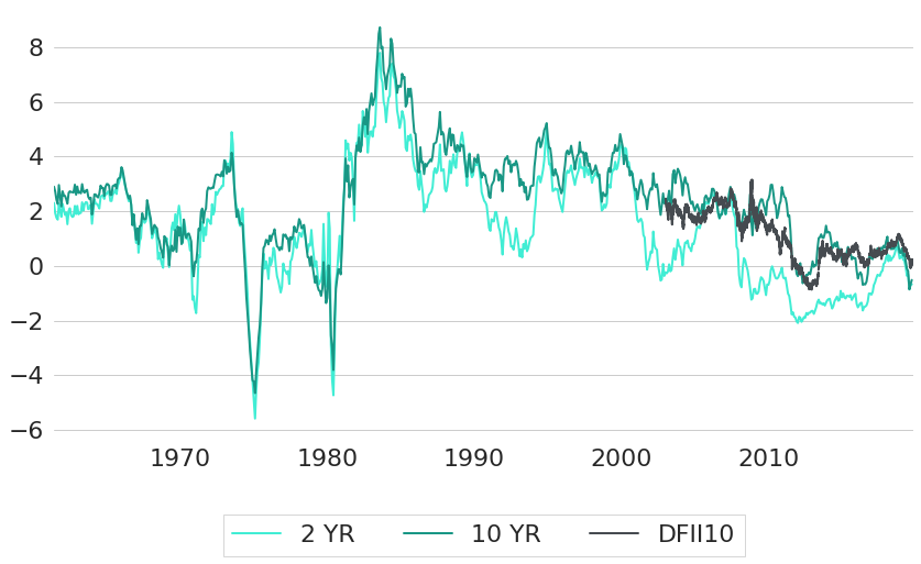
Figure 6: Historic Real Rates
In Figure 3 we have already seen how the short end of yield curves is largely driven by the Effective Federal Funds Rate. However, we can also see that this does not equally hold for long-term interest rates which follow the FED target rate less closely. In general, long-term interest rates tend to be higher than short-term rates, because when you commit to lend money for a longer period of time, you usually also have to face higher risks than for shorter periods. As we will see in more detail in subsequent blog posts in this series on fixed-income securities, bonds with long durations are more sensitive to interest rate changes, because changing interest rates will just change the discounting rates on more cash-flows that are further in the future. The higher compensation required for long-term commitments is also called the liquidity premium. However, even though financial market participants usually require more compensation for longer durations, the actual level of compensation nevertheless fluctuates over time quite significantly. This can be seen in Figure 7 which shows the difference between 10 year and 1 year CMT rates over time (also called the "slope" of the yield curve). As we can see, most of the time the line is above zero, because long-term rates are usually higher than short-term rates. However, at some specific points in time this relationship does invert and short-term rates have actually been higher than long-term rates, which is shown by the line being below zero. In these situations one speaks of an "inverted" yield curve. The presence of an inverted yield curve with negative liquidity premium on long-term rates is actually such an abnormal situation that it is usually an indicator of more fundamental distortions in financial markets and as such has been a good predictor of US recessions which are indicated by the grey colored bars in the background of the chart. As we can see, every US recession in the last 60 years has been preceded by a period of inverted yield curves10.
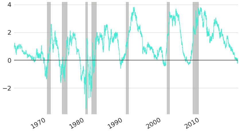
Figure 7: Yield Curve Slopes (10 Year minus 1 Year CMT Rates) and US Recessions
Until now we have only looked at US Treasury rates, because publicly available data goes back much further than for the EU area. From the ECB we can obtain a dataset for EU government interest rates similar to what we have for US Treasury rates: daily parameter estimates of a Svensson yield curve model, estimated for EU Government bonds with AAA rating11. The data goes back until the end of 2004, and yield curve parameters again can be converted into constant maturity rates. Figure 8 shows constant maturity rates for some selected maturities over time. In contrast to US rates, EU rates actually did cross the line into negative territory in 2015, remaining below zero until the time of writing. At the end of the sample rates are even negative for almost all shown maturities.
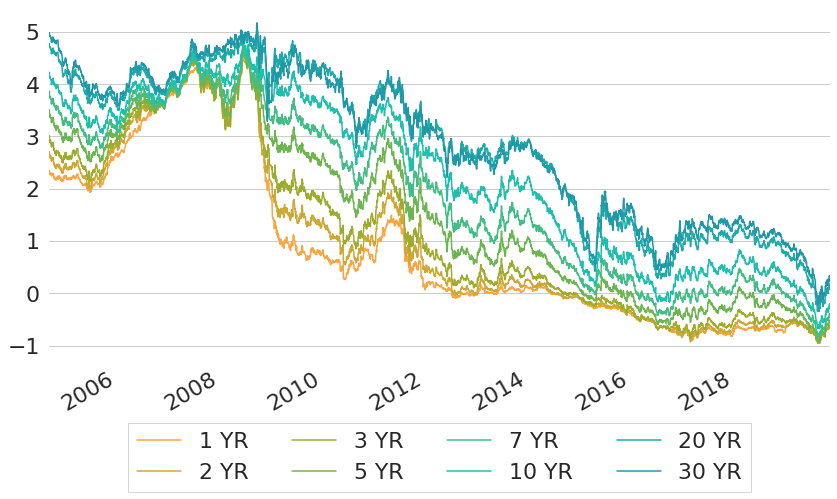
Figure 8: Constant Maturity Rates for EU Government Bonds with AAA Rating
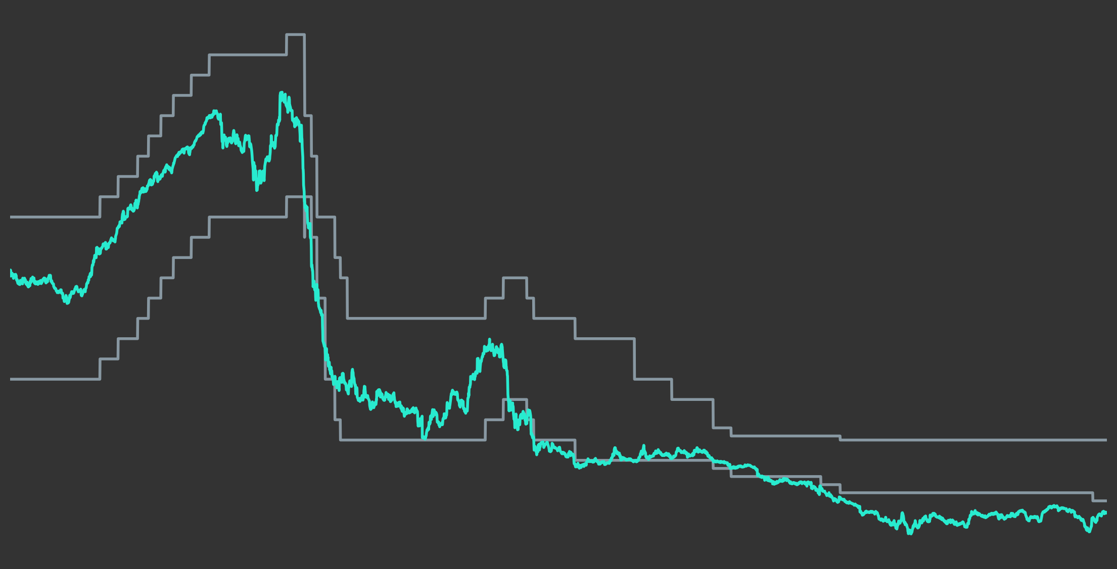
Similar to the US, the short end of the yield curve is driven by central bank decisions in the EU as well. Figure 9 shows constant maturity rates of maturity one year, together with so-called ECB deposit (DFR) and marginal lending facility rates (MLFR). Deposit facility rates define the interest that banks receive when they deposit money with the ECB overnight, marginal lending facility rates are the rates at which banks can borrow overnight from the ECB. Both these rates are set every six weeks by the ECB and hence are piecewise constant. As we can see from the chart, short-term interest rates are essential driven by these two rates.
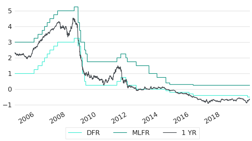
Figure 9: ECB Standing Facilities and Short-Term Yields
So far we have seen that interest rates in both the US and EU are significantly driven by central banks at their short end and how both have evolved over time in the past. Last but not least, Figure 10 shows how official central bank rates of both regions tend to move together over time.
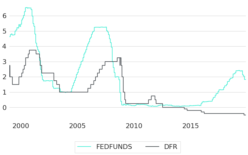
Figure 10: EU and US Central Bank Rates
Both US Government rates as well as EU Government rates for countries with AAA rating are usually perceived to be almost free of credit risk. Without credit risk, you will always get back your principal as well as all coupon payments that have been promised to you by your counterpart. However, many bonds do have a non-negligible probability of default, such that financial market participants require a compensation for the credit risk involved. This means that they either require higher coupon payments, or they are only willing to pay less for any given promised series of future cash-flows, because some of these future cash-flows might actually never get paid. This characteristic of the asset pricing process for bonds with credit risks is reflected in higher interest rates: market participants require an additional spread on top of risk-free rates. One way to see this is by looking at yields of different corporate bonds in comparison to risk-free government bond yields. Figure 11 shows constant maturity rates of US government bonds with 20 year maturities together with yields for corporate bonds of two different credit qualities: AAA and BAA rated bonds. Data for both corporate bond yields is from Moody's and provided by FRED12. These yields are based on bonds with maturities of 20 years and above, hence the comparison to CMT rates with 20 years maturity. As economic theory suggests, corporate bond yields are higher than US government yields at basically all points in time. Even AAA rated bonds already traded at a small spread compared to government yields, and BAA rated bonds just exhibit even higher rates.
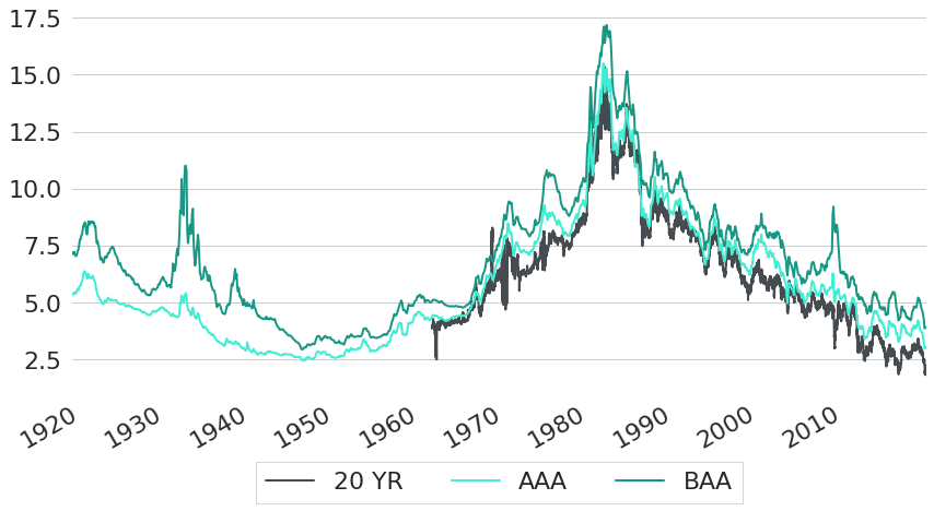
Figure 11: Historic US Corporate and US Government Yields for Long Maturities
A similar conclusion we also can get for bonds with shorter maturities. Figure 12 shows a comparison of the ICE BofAML US High Yield Master II Effective Yield (BAMLH0A0HYM2EY)13 and government bond yields. The ICE US High Yield relates to USD denominated corporate debt with a rating below investment grade, and issuance in the US domestic market. It is a capitalisation-weighted basket of fixed-income securities with remaining maturity greater than 1 year. From the chart we can see that the spread between US government and corporate bond yields significantly varies over time. While the spread was roughly 2.5% at the end of 2007, it increased to more than 15% at the peak of the Global Financial Crisis of 2008 / 2009. This, however, does not mean that expected returns of US corporate bonds were more than 15% larger than for US government bonds. The additional yield of bonds with credit risk could only be fully harvested if one actually receives all promised future cash-flows. This would be tantamount to a case of zero defaults which is highly unlikely in the case of the ICE US High Yield, given that it consists of securities with ratings below investment grade. In other words: the ex-ante corporate bond yields are larger than the actually expected returns and the difference between yields and returns is caused by losses due to defaults.
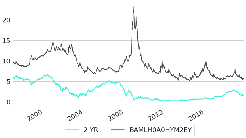
Figure 12: Historic US Corporate and US Government Yields for Medium Maturities
Credit spreads are also a popular indicator for the amount of credit risks in an economy. For example, the so-called TED spread (or TED rate) measures the spread between 3-month LIBOR based on US dollars and 3-month Treasury Bill rates. Historic values of the TED spread (TEDRATE14 are shown in Figure 13. The maximum value of the time series occurred during the Global Financial Crisis of 2008 / 2009.
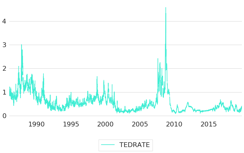
Figure 13: TED Spread
Credit risk is not only a characteristic of corporate bonds, but also government bonds of countries with high levels of debt or other economic vulnerabilities could be subject to defaults and hence generally have higher interest rates than governments with highest creditworthiness. One example to see this is by looking at long-term yields (maturities of close to ten years15) of several European government bonds as shown in Figure 14. Although interest rates of most countries follow a similar trend of decreasing interest rates, some individual countries traded at significantly higher yields in the past.
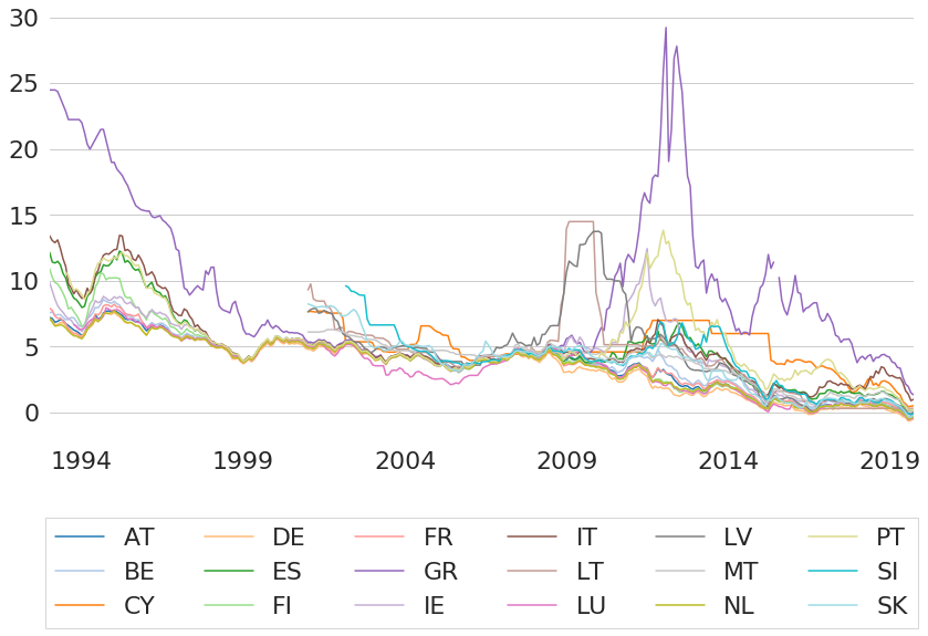
Figure 14: Historic EU Government Country Bond Yields
Looking at yields of different countries today (Figure 15) we can also see the wide variations in yields. For example, Greece government bonds of ten year maturity currently trade at a yield of slightly above 1.25%, while German government bonds only trade at a negative yield of almost -0.5%. This is the lowest value of all the selected countries, but it is not the only one with interest rates in negative territory: roughly half of the countries currently have interest rates below zero.
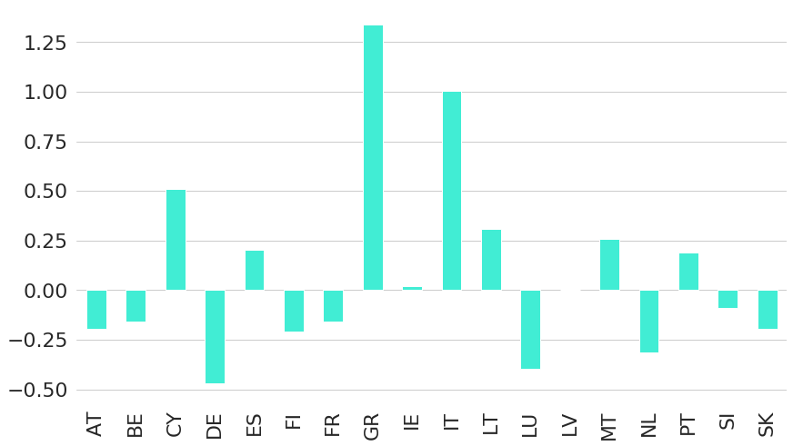
Figure 15: Current EU Government Country Bond Yields
Gurkaynak, Refet. S., Sack, Brian, and Wright, Jonathan H. (2006), The U.S. Treasury Yield Curve: 1961 to the Present, Federal Reserve Board Finance and Economics Discussion Series.
Svensson, L. E. O. (1994), Estimating and Interpreting Forward Rates: Sweden 1992-4, National Bureau of Economic Research Working Paper #4871.
Uribe, M. (2018), The Neo-Fisher Effect: Econometric Evidence from Empirical and Optimizing Models, National Bureau of Economic Research Working Paper #25089.
1 Daily Treasury Yield Curve Rates Resource Center
2 https://fred.stlouisfed.org/series/FEDFUNDS
3 https://www.chicagofed.org/research/dual-mandate/dual-mandate#note1
4 https://fred.stlouisfed.org/series/CPILFESL
5 https://data.worldbank.org/indicator/FP.CPI.TOTL.ZG
6 https://data.worldbank.org/indicator/fr.inr.lend
7https://data.worldbank.org/indicator/fr.inr.risk
8 https://fred.stlouisfed.org/series/DFII10
9 https://fredblog.stlouisfed.org/2014/04/long-run-inflation-expectations/
10 For further details on this topic you can listen to the Meb Faber Show podcast episode with Cam Harvey: https://mebfaber.com/2019/08/28/episode-172-cam-harvey-this-is-a-time-of-considerable-risk-of-a-drawdown/
11 Data is available under the Financial market instrument ticker G_N_A (e.g. YC.B.U2.EUR.4F.G_N_A.SV_C_YM.BETA0) at the ECB Yield curves section of the Statistical Data Warehouse: http://sdw.ecb.europa.eu/browse.do?node=9691126
12 https://fred.stlouisfed.org/series/AAA, https://fred.stlouisfed.org/series/BAA
13 https://fred.stlouisfed.org/series/BAMLH0A0HYM2EY
Disclaimer – The views and opinions expressed in this blog are those of the author and do not necessarily reflect the views of Scalable Capital Bank GmbH, its subsidiaries or its employees ("Scalable Capital", "we"). The content is provided to you solely for informational purposes and does not constitute, and should not be construed as, an offer or a solicitation of an offer, advice or recommendation to purchase any securities or other financial instruments. Any representation is for illustrative purposes only and is not representative of any Scalable Capital product or investment strategy. The academic concepts set forth herein are derived from sources believed by the author and Scalable Capital to be reliable and have no connection with the financial services offered by Scalable Capital. Past performance and forward-looking statements are not reliable indicators of future performance. The return may rise or fall as a result of currency fluctuations. Please refer to our risk information.
Risk Disclaimer – There are risks associated with investing. The value of your investment may fall or rise. Losses of the capital invested may occur. Past performance, simulations or forecasts are not a reliable indicator of future performance. We do not provide investment, legal and/or tax advice. Should this website contain information on the capital market, financial instruments and/or other topics relevant to investment, this information is intended solely as a general explanation of the investment services provided by companies in our group. Please also read our risk information and terms of use.