Leveraged Indices and the Volatility Drag

12. April 2019 | Dr. Christian Groll

Disclaimer – The views and opinions expressed in this blog are those of the author and do not necessarily reflect the views of Scalable Capital GmbH or its subsidiaries. Further information can be found at the end of this article.

Summary

Leveraged indices are a tool to increase exposure to certain indices. They come with higher risk, but also higher return potential than the original underlying index itself.
Leverage can be established by borrowing money in order to increase the investment into an index.
Leveraged indices are constructed from net total return indices by scaling of the returns of the underlying index and subtracting borrowing costs.
Knowledge of the construction methodology of a leveraged index allows computation of leveraged index trajectories for any given price trajectories of the underlying index.
In a simulation study we analyse how leverage will change the payoff distribution of the underlying index.

Construction of Leveraged Indices

In this post we want to examine leveraged indices. The idea of leveraged indices is to increase the exposure to a certain index. Hence, a leveraged index should come with higher risks but also higher return potential than the original underlying index itself.

First, we show how leveraged indices can be constructed manually. The idea behind leveraged indices is quite simple: One just needs to duplicate the original investment into a certain index. Hence, one does not simply buy the underlying index once, but through borrowing of additional money one buys into a certain market multiple times. For a leverage factor of 2 and an initial investment of €100 this means: Borrow additional €100 and invest the total amount of €200 into the index. Borrowing money will come at the expense of costs, in the form of interest rate payments.

Normalized prices for EURO STOXX 50 Net Return Index

Figure 1: Normalised prices for EURO STOXX 50 Net Return Index

Figure 2: EONIA rates (in percentage points)

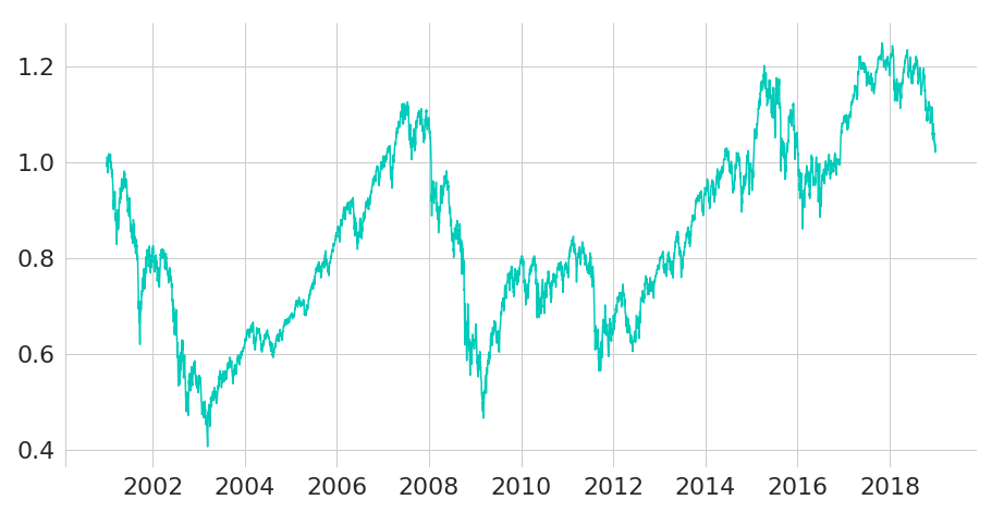
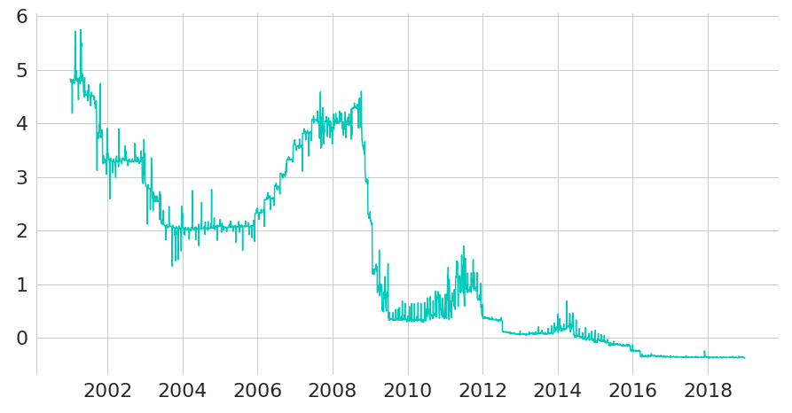
We will now manually compute the trajectory of a daily leverage index on the EURO STOXX 50, where we assume that borrowing can be done at EONIA rates. The following charts show normalised prices for the EURO STOXX 50 Net Return Index (SX5T Index) in Figure 1 and EONIA rates (in percentage points) in Figure 2. All data is taken from Bloomberg, ranging from January 2000 until the end of 2018.

When manually computing leveraged index returns we will apply the following index methodology:

Daily leverage index methodology

Let $R$ denote the total return of the underlying index between two dates $t-1$ and $t$ , and $r_{ov}$ denote the annualised rate of borrowing (we will simply use the overnight rate for this). Furthermore, let $g$ denote the leverage ratio (or leverage factor), and $T$ denote the number of calendar days between dates $t-1$ and $t$ . Then the leverage daily index total return $R_L$ is defined by (e.g. see the leverage index methodologies of MSCI, STOXX or S&P):

R_L=g cdot R +(1-g) cdot r_{ov} cdot frac{T}{360}

For the sake of simplification we will allow the following two imprecisions:

In reality, $T$ can be 1 day during business weeks, 3 days for Friday to Monday returns, and even something else depending on holidays. On average, however, with roughly 250 index returns per year, the borrowing rate has to be paid for $frac{1}{250}$ days.
If $R$ denotes the index return from $t-1$ to $t$ , then we need to subtract the borrowing rate prevailing in $t-1$ .

Daily returns of the leverage index with $g=2$ hence can be computed as follows:

lev_2x_daily_rets = equ_data['SX5T Index'].pct_change()
lev_2x_daily_rets = lev_2x_daily_rets * 2 - eonia['EONIA Index']/100 * 1/250

# aggregate daily returns to an index performance
lev_2x_daily_perfs = (lev_2x_daily_rets + 1).cumprod()

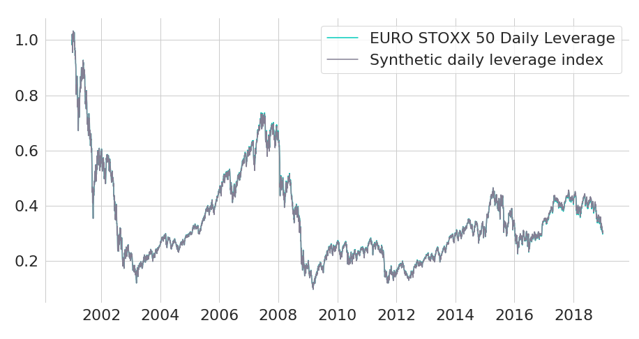
Normalized EURO STOXX 50 Daily Leverage Net Return Index compared to synthetic index replication

Figure 3: Normalised EURO STOXX 50 Daily Leverage Net Return Index compared to synthetic index replication

We can now compare the true index values of EURO STOXX 50 Daily Leverage Net Return (SX5TL Index) with our manually computed index. Due to the simplifications that we made we will not end up replicating the leveraged index with full accuracy. Hence, we will label our manually computed index as "synthetic".¹ Both EURO STOXX 50 Daily Leverage Net Return and our synthetically computed index is shown in Figure 3. For simplicity, we normalize the performance of both indices to one on the start date. As you can see, both lines are matching so closely that the synthetic index line is almost not visible.

Constant borrowing costs

Now let's also examine another inaccuracy during index computation: Instead of using true daily prevailing EONIA rates we now use a constant borrowing rate equal to the average EONIA rate of the whole sample period. Only now will differences between the manually computed version of the leveraged index and the Bloomberg time series become visible.

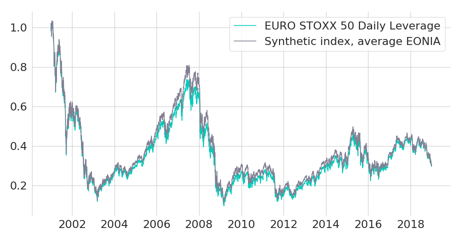
Normalized EURO STOXX 50 Daily Leverage Net Return Index compared to synthetic index replication with average borrowing costs

Figure 4: Normalised EURO STOXX 50 Daily Leverage Net Return Index compared to synthetic index replication with average borrowing costs

Even this rather intrusive simplification does not really change the macro characteristics of the leveraged index. When simulating leveraged index paths further below we will hence rely on the simplifying assumption of constant borrowing rates.

Monthly leveraged indices

Instead of applying the desired leverage factor on a daily basis, one could also reset the leverage ratio less frequently. For example, monthly leveraged indices only calibrate the desired leverage ratio at the beginning of each month, such that the leverage ratios in between will vary, subject to market moves. In this case, one cannot borrow at EONIA overnight rates anymore, because the money will be needed for a full month.

Realised Risk-Return Profiles

Now that we have a basic understanding of how leveraged indices are constructed, let's further examine the impacts of leveraging. Using a leverage factor of 2 we get roughly 2 times the daily return of the underlying index each day. But what does that mean in the long run? Should we expect to get twice the return here as well?

To answer this question, let's first compare the performances of the EURO STOXX 50 Index with daily and monthly leverage indices. In addition, we also show a synthetic time series that for each day is computed as twice the performance of the EURO STOXX 50 Index. So if the EURO STOXX 50 Index has an aggregate performance of 12% at a given day, then the synthetic time series will show a value of 24%. This time series shall represent the target multiple (in our case a factor of 2) by showing the values that one might be inclined to expect by naively applying the leverage factor of 2 to longer time periods.

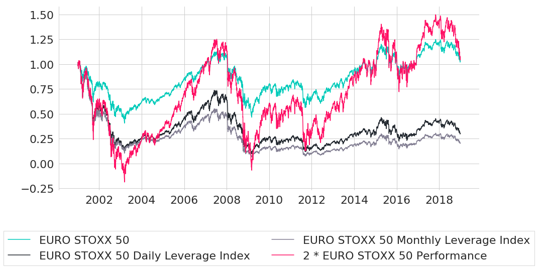
Leverage indices compared to regular performance of index & re-scaled performance

Figure 5: Leverage indices compared to both regular performance of underlying index and re-scaled performance that is obtained by multiplication with target multiple

As we can see, while the EURO STOXX 50 Index did have a slightly positive performance over the given time period, both leverage indices result in a strong negative performance. The long-term performance of both leveraged indices hence deviate significantly from the performance that one might expect by naively applying the leverage factor to longer time horizons. So how can that be?

First of all, the chart already indicates a crucial flaw in the naive multiplication logic: the synthetic time series takes on values below zero in 2003. Obviously, this is not possible, as prices cannot fall below zero (if they really reached zero at some point, then this would be a final state as the time series could never recover again).

The differences between true leveraged index performance and the synthetic and naive computation is caused by compounding effects and is sometimes referred to as volatility drag. In the long run, leveraged indices tend to deviate from the targeted multiple significantly. In terms of risk, however, both leveraged indices seem to keep their promise: annualised volatility (using simple square root of time scaling on daily returns) is roughly two times the level of the underlying index, whilst the maximum drawdowns are significantly worse:

Metric	EURO STOXX 50	Daily Leverage	Monthly Leverage
Annualised return	0.21	-6.33	-8.32
Annualised volatility	23.22	46.46	48.05
Maximum drawdown	60.04	90.57	93.75

Table 1: Risk and return metrics

Effects of Leveraging on Payoff Distributions

Let's now analyze how this volatility drag distorts the targeted performance and whether it systematically works against the investor. Since we already know how to manually compute leveraged index values given the trajectory of the underlying index, we can easily analyze the effects of the volatility drag in a simulation study. For the sake of simplicity, we will assume constant borrowing costs equal to the average EONIA rate, as we already have seen that this should not have a major impact on results. Furthermore, we use the following settings for the simulation study:

Regular index performances following a Brownian motion: For logarithmic returns we assume an annual compounding of 6%, while the standard deviation is chosen to match the volatility of logarithmic returns of the EURO STOXX 50 index time series.
Simulation of 2000 paths, each of length 5000 (corresponding to roughly 20 years with 250 business days per year).
A leverage factor equal to 2.

# specify costs of borrowing
avg_eonia = eonia.mean().squeeze()

# set parameters of normal distribution of logarithmic returns
log_mu = 0.06 / 250
log_rets = np.log(data['SX5T Index'].pct_change() + 1)
log_sigma = log_rets.std()

# specify leverage factor and scale of simulation study
n_reps = 2000
n_obs = 5000
lev_fact = 2

# set random seed for reproducibility
np.random.seed(9001)

# preallocate output
all_normal_perfs = np.empty([n_obs, n_reps], dtype=float)
all_lev_perfs = np.empty([n_obs, n_reps], dtype=float)

for ii in range(0, n_reps):
    # draw random innovations
    log_innovs = np.random.normal(loc=log_mu, scale=log_sigma, size=n_obs)

    # compute regular index performance
    disc_gross_rets = np.exp(log_innovs)
    sim_perfs = np.cumprod(disc_gross_rets)

    # compute leverage index performance
    disc_net_rets = disc_gross_rets - 1
    disc_rets_lev = disc_net_rets * lev_fact + (1-lev_fact) * avg_eonia/100 * 1/250
    sim_lev_perfs = np.cumprod(disc_rets_lev + 1)
    
    # store simulated paths
    all_lev_perfs[:, ii] = sim_lev_perfs
    all_normal_perfs[:, ii] = sim_perfs

Figure 6: Simulated index trajectories for underlying index and leverage index

Selected simulated index trajectories for one bad, one moderate and one good outcome of the underlying index

Figure 7: Selected simulated index trajectories for one bad (top), one moderate (middle) and one good outcome (bottom) of the underlying index

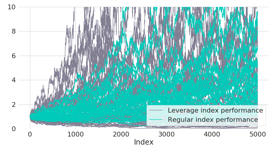
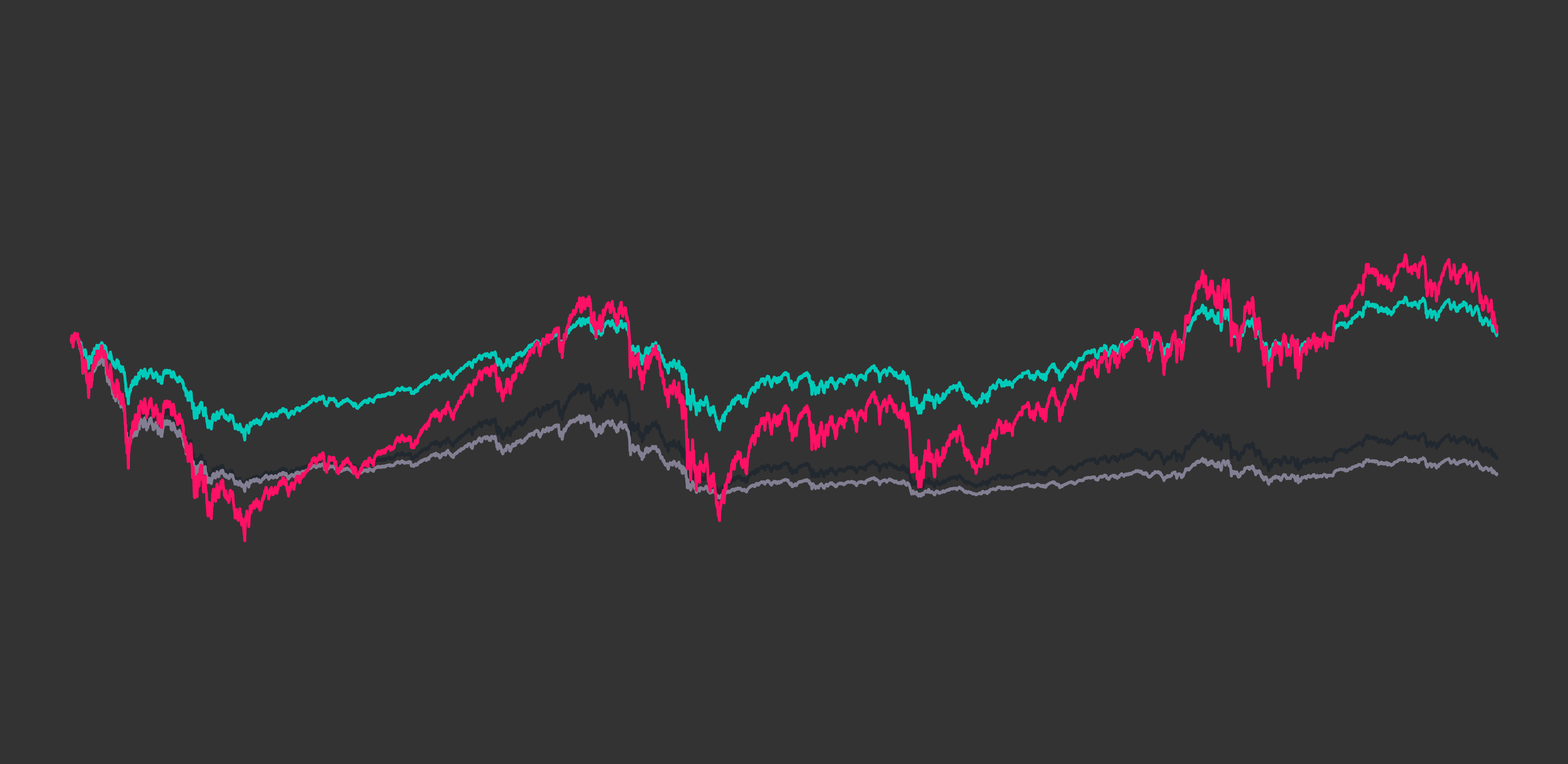
To get an impression of the simulated paths, Figure 6 plots the first 50 paths for both the regular index and leveraged index. Regular index paths are plotted on top, such that the more volatile paths of the leveraged index can be seen in the background.

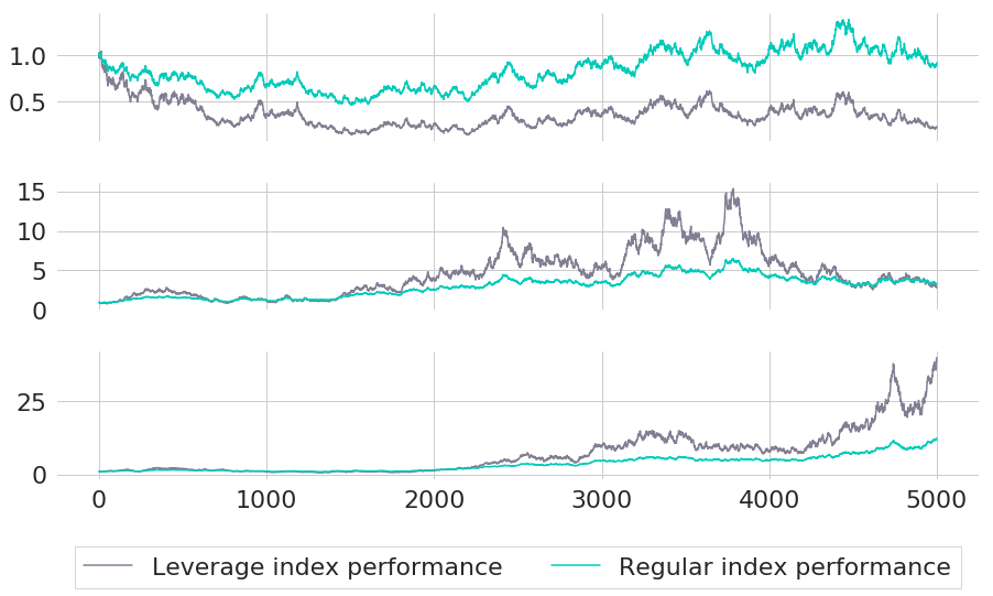
To get a more detailed view on the differences between regular and leveraged index paths we now compare both versions for three selected scenarios in Figure 7:

The regular index paths that mark the performance of both the quantile of the 10% lowest and highest overall performance.
The regular index path that marks the median performance of all simulated paths.

The uppermost chart represents trajectories for the 10% quantile of regular index outcomes. In other words, it represents a rather bad outcome - only in 10% of all scenarios the regular index has an outcome that is even worse. As we can see, the almost flat overall performance of the regular index translates into a loss of roughly 75% for the leveraged index. Again, the leveraged index performance is far from the naive target multiple of 2. Even for the median case, the leveraged index does not give the desired amplification of the positive index performance - both indices end at roughly equal levels. This is quite a disappointing outcome, given that we hoped to achieve a multiple of 2 on the regular index performance that has an annualised return (in percentage points) of 6.14. Only in the bottom chart of Figure 7 the leveraged index really leads to a significantly better performance. Instead of an annualised return of 13.34 for the regular index, the leverage index achieves 20.21 percent annualised.

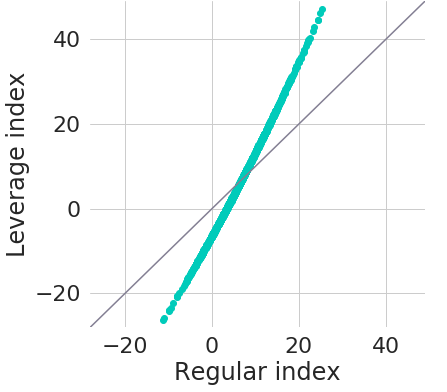
Figure 8: Comparison of annualised returns (%) for simulated paths of underlying index and leverage index

We can also obtain a similar comparison for all simulated scenarios simultaneously. Figure 8 shows annualised performance of regular index paths on the x-axis and annualised performance of leveraged index paths on the y-axis. The black diagonal line represents the cases where both indices would have the same performance.

As we can see from the chart, the leveraged index only results in better performance for scenarios above roughly 7% annualised return for the regular index. Or, looking at it from a different perspective: the leveraged index outperforms the regular index in 44.4% of all cases.

¹ This term is usually used for funds that try to replicate some underlying index without actually physically owning the underlying securities. It matches in our case, as we also want to achieve exposure to an available leveraged index without directly investing into it, but by replicating it manually.

Disclaimer – The views and opinions expressed in this blog are those of the author and do not necessarily reflect the views of Scalable Capital GmbH, its subsidiaries or its employees ("Scalable Capital", "we"). The content is provided to you solely for informational purposes and does not constitute, and should not be construed as, an offer or a solicitation of an offer, advice or recommendation to purchase any securities or other financial instruments. Any representation is for illustrative purposes only and is not representative of any Scalable Capital product or investment strategy. The academic concepts set forth herein are derived from sources believed by the author and Scalable Capital to be reliable and have no connection with the financial services offered by Scalable Capital. Past performance and forward-looking statements are not reliable indicators of future performance. The return may rise or fall as a result of currency fluctuations. Please refer to our risk information.

Risikohinweis – Die Kapitalanlage ist mit Risiken verbunden und kann zum Verlust des eingesetzten Vermögens führen. Weder vergangene Wertentwicklungen noch Prognosen haben eine verlässliche Aussagekraft über zukünftige Wertentwicklungen. Wir erbringen keine Anlage-, Rechts- und/oder Steuerberatung. Sollte diese Website Informationen über den Kapitalmarkt, Finanzinstrumente und/oder sonstige für die Kapitalanlage relevante Themen enthalten, so dienen diese Informationen ausschließlich der allgemeinen Erläuterung der von Unternehmen unserer Unternehmensgruppe erbrachten Wertpapierdienstleistungen. Bitte lesen Sie auch unsere Risikohinweise und Nutzungsbedingungen.

Dr. Christian Groll

Chief Investment Officer (Ehemals)

Christian ist Chief Investment Officer von Scalable Capital. Er kam 2015 als Mitglied des Financial-Engineering-Teams ins Unternehmen und war von 2018 bis 2021 Head of Quantitative Investment Strategy. Christian hat einen Doktortitel in Statistik und verfügt über Expertise in den Bereichen Quantitative Finance, Portfolio-Management und in der Modellierung von Finanzmarktrisiken. Vor seiner Zeit bei Scalable Capital verbrachte er sechs Jahre in der Forschung an der Ludwig-Maximilians-Universität (LMU) in München. Während dieser Zeit promovierte er zum Thema „Dynamic Risk Management of Multi-asset Portfolios“. Christian hat Wirtschaftsmathematik an der LMU studiert.

Die Kapitalanlage ist mit Risiken verbunden. Der Wert Ihrer Kapitalanlage kann fallen oder steigen. Es kann zu Verlusten des eingesetzten Kapitals kommen. Frühere Wertentwicklungen, Simulationen oder Prognosen sind kein verlässlicher Indikator für die künftige Wertentwicklung. Bitte beachten Sie hierzu unsere Risikohinweise.

Für Neukunden: 4 % p.a. Zinsen (Baader Bank) bis 1 Mio. € für 4 Monate. Danach 2,6 % p.a. variabler Zins bis 100.000 €. Zinsangebot nur mit PRIME+. Mehr Informationen.

Folgen Sie uns

Newsletter abonnieren

Scalable Capital GmbH
Seitzstraße 8e, 80538 München | Kontakt | Impressum
Zuständige Aufsicht: BaFin, Deutsche Bundesbank