Risks of Long-Term Stock Market Investments
August 2, 2019 |
Disclaimer – The views and opinions expressed in this blog are those of the author and do not necessarily reflect the views of Scalable Capital Bank GmbH or its subsidiaries. Further information can be found at the end of this article.
According to survey data roughly only 16% of people in Germany own stocks or funds that invest in stocks (e.g. see the Aktionärszahlen des Deutschen Aktieninstituts). From personal experience I would say that far too many people perceive stocks to be more risky than they really are. Yes, even the larger stock market indices can experience drawdowns greater than 50%. But if you have a broad and well-diversified portfolio and stick with your investment, these losses are only temporary, stock markets will recover again and they will achieve outstanding performance results in the long run.
Like the old gym saying "no pain, no gain" there is a similar saying for stock markets: "no pain, no premium". The idea behind this saying is that stock markets deliver such outstanding returns only because they are required by investors as compensation for the risks that come along. In other words: if there were no risks involved, there also would be no returns in excess of the risk-free rate. People require the prospect of future excess returns in order to be willing to participate in investments that bear risk. This is a very important concept that everyone should keep in mind: risks are the currency that investors need to pay in order to get excess returns in the long run. So the higher the risks, the higher the returns that we should demand as compensation. Still, the question remains: how high should the compensation for any additional unit of risk be? And how does this trade-off between risks and compensation look like for stock returns?
In order to find an answer to these questions, let's do a quick analysis based on historic stock market data. For the analysis we will use the US stock market index provided by Fama and French. The index is publicly available on a daily basis, goes back to 1926 and represents a value-weight return of all CRSP firms incorporated in the US and listed on the NYSE, AMEX, or NASDAQ.
First we download Fama-French factor data from the Kenneth French data webpage. Market returns are given as excess returns in the dataset, so to get nominal market returns we need to incorporate risk-free rates.
ff_factors = web.DataReader('F-F_Research_Data_Factors_daily', 'famafrench', start='1910')

# display the data description
print(ff_factors['DESCR'])

# compute nominal market return from excess returns
ff_factor_rets = ff_factors[0]
ff_factor_rets['Mkt'] = ff_factor_rets['Mkt-RF'] + ff_factor_rets['RF']
ff_market_rets_pct = ff_factor_rets['Mkt']

# compute market performance from returns
ff_market_perf = (ff_market_rets_pct / 100 + 1).cumprod()

 > F-F Research Data Factors daily
 > -------------------------------
 >
 > This file was created by CMPT_ME_BEME_RETS_DAILY using the 201904 CRSP database.
 > The Tbill return is the simple daily rate that, over the number of trading days
 > in the month, compounds to 1-month TBill rate from Ibbotson and Associates Inc.
 > Copyright 2019 Kenneth R. French
 >
 >   0 : (24473 rows x 4 cols)
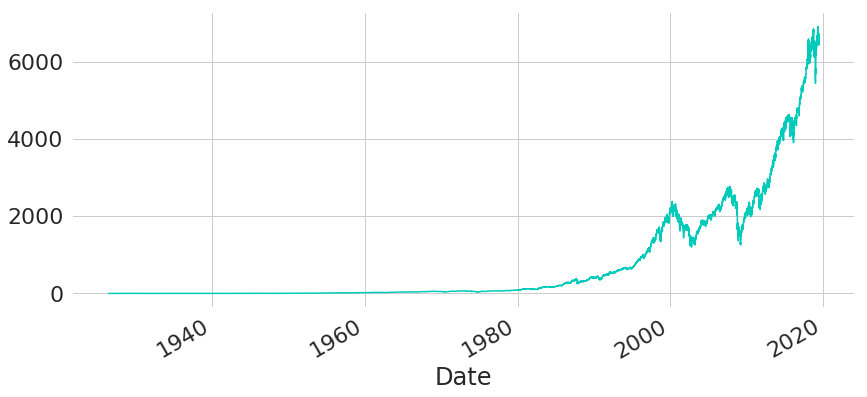
Over the long run the US market achieved an annualised return of almost 10%. Given this large annualised return and the effects of compounding, 1 USD invested on 1926-07-01 would have increased to more than 6500 USD by the end of May 2019.
Through compounding, an investment with steadily re-invested distributions will increase exponentially, as any gains of previous periods will again compound similar to the initial investment itself. For longer periods (multiple decades) this effect usually has such a strong impact that any patterns in the beginning of the investment period are not visible anymore in a regular performance chart. The scale at which value changes happen (measured in absolute terms of USD) simply becomes too different over time.
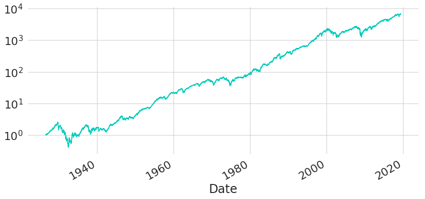
The increase in value does not happen constantly over time, but investments in financial markets come with huge fluctuations. However, due to the large effects of long-term compounding the majority of the line chart (the first part of it) looks almost flat. Only on a logarithmic scale we can see that fluctuations did occur here as well and that the time series has equal patterns over the full period. With a logarithmic axis, equal percentage moves are represented by changes of constant amount on the y-axis.
Hence, a 20% move of a still tiny portfolio at the very beginning of the sample will cause the same change on the y-axis as a 20% move of an already large portfolio at the end of the sample. With a logarithmic scale we can better see the trajectory of market performance in the beginning of the sample. In particular, we can see how market performance crucially dropped during the Great Depression, where it took many years to fully recover from the market downturn. Overall, this meant approximately 15 years without a new all-time high and hence without any increase in value for someone who was already invested before the last all-time high.
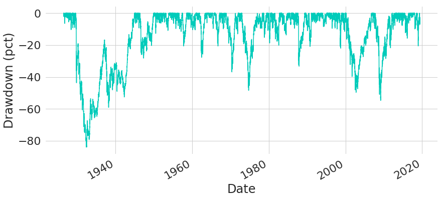
An even better way to see the magnitude of market downturns is by looking at drawdowns. Drawdown measures the percentage decrease in value with regards to the previous all-time high. Looking at the drawdowns of the market index we can see that an investor would have temporarily lost more than 80% if they had been unfortunate and first invested exactly at the all-time high previous to the Great Depression. But this would not have been the only unsettling market downturn that an investor would have had to endure: drawdowns of more than 30% have happened on multiple occasions over the decades.
Looking at these huge risks, it's no surprise that some people might be afraid of the stock market. However, when the market goes down, it is not like all the money has disappeared into thin air. If you don't sell and realise your losses, it might just be a temporary drop in value which is recovered once the market goes up again afterwards. So the question is: should we trust markets to always recover and how long do we need to wait until prices have recovered? Let's look at our historic data again, this time through the perspective of return triangles.
Return triangles are a tool to visualise realised (annualised) returns of multiple subperiods. In our first example below, we show a return triangle for the Fama-French market index with data from 1990 to end of May 2019. The return triangle is based on yearly data and shows for each possible subperiod the realised annualised return of the market index. Any investment subperiod is given by a buying date (the beginning of the subperiod) and a selling date (the end of the subperiod). Buying dates are given by the axis on the right, selling dates are given by the axis on the top. The left-most diagonal shows the shortest subperiods (in this case periods of one year as we are working with yearly data). Moving on to the next diagonal, we can read off all subperiods with length equal to two years, and the further we go to the upper right, the longer the subperiods will get, until eventually we reach the longest period that simply represents the full period in the upper right corner. To help identify subperiods of any particular length, the chart also shows two auxiliary border lines in turquoise. In this case they highlight the diagonals that represent all 10 year and 20 year holding periods. For further details and also the Python computer code to create such charts yourself please take a look at our blog post A Python Implementation of Triangles for Visualising Long-Term Investment Metrics.
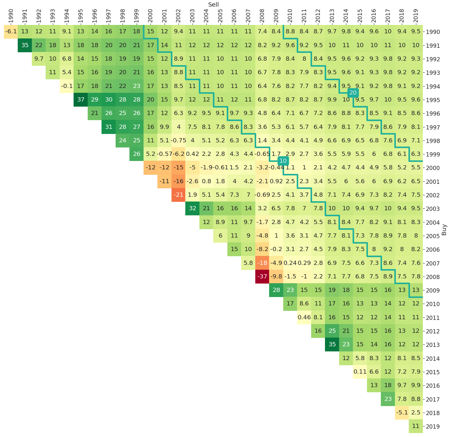
So what can we learn from the chart? Let's start by looking at short subperiods of only one year shown on the left-most diagonal. For such short periods investing can be viewed as a matter of luck. In bad years like 2008 you lost 37% of your investment, while you would have gained 37% in a single year in 1995. The only problem is: you won't be able to tell whether it is a good year or a bad year in advance, so that short-term investing becomes a matter of timing luck. Even when we move to slightly longer periods of three years there still is a huge variation of results. Investing from beginning of 2000 to end of 2002 resulted in annualised losses of 15%, while the three year period from 1995 to 1997 achieved gains of 30% annualised. But once we move to subperiods longer than 10 years we can see that not a single annualised return is negative anymore. With such long holding periods the general upwards trend kicks in and dominates the market index trajectory even if the subperiod includes major market downturns like the Financial Crisis of 2008 or the bursting of the Dot-com bubble in 2000.
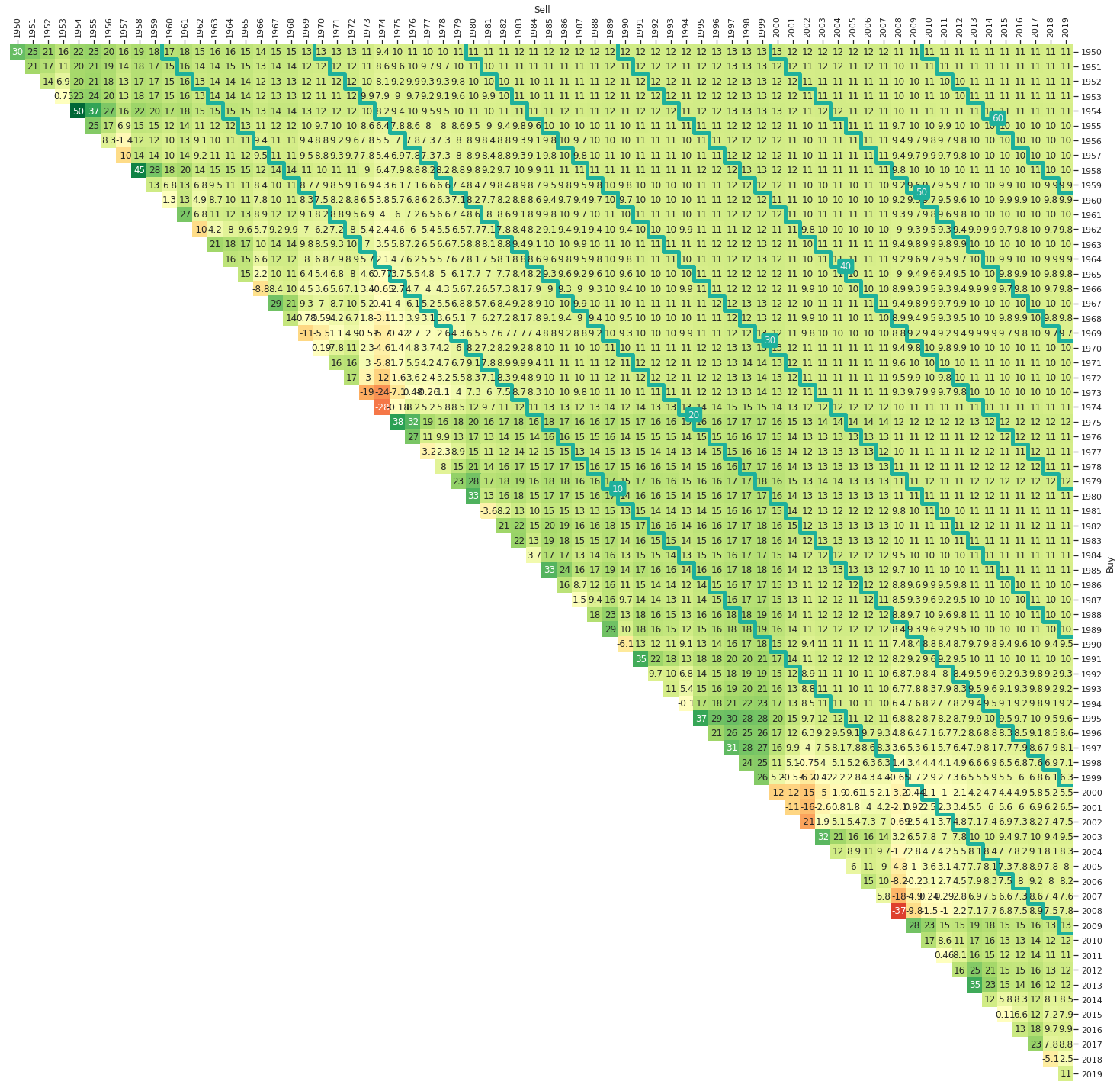
Now that we know how to interpret return triangle charts let's increase the overall sample period back to 1950. The triangle chart becomes even larger and some numbers will be hard to read but even from the colour coding it becomes clear that there are no negative annualised return periods anymore for holding periods above 10 years.
The market index goes back even further than 1950, but showing even more periods in a triangle chart makes it a bit too crowded. One alternative visualisation is the following chart that only uses two colours in order to distinguish between periods with positive and negative annualised returns. This way we can visualise the full history of the market index.
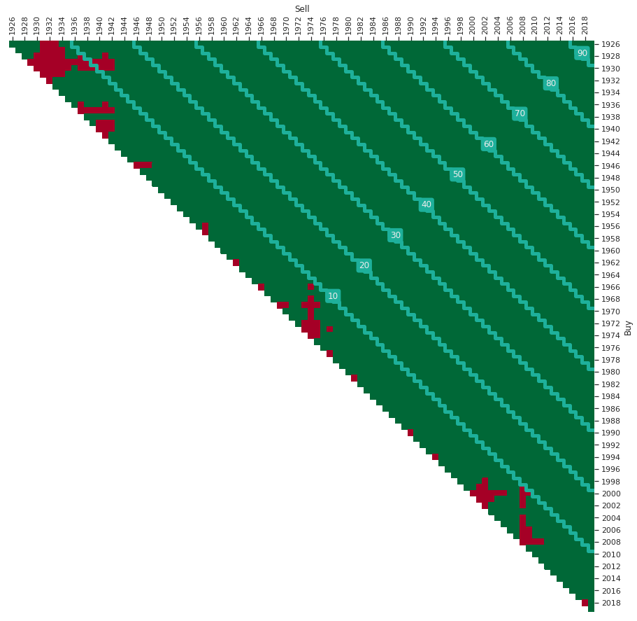
Now we can see: during the Great Depression of the 1930s there are holding periods above 10 years that nevertheless had negative annualised returns (shown as red tiles). Still, never in the history of the market index there was a subperiod of 15 years or above where there was a negative result. In other words: if you just held your investment for long enough then you would never have lost money with this market index.
This is not to say, however, that you are not exposed to timing luck. Variations of returns can still be huge. For your end wealth it matters tremendously whether you achieve annualised returns of 2% or 6% over a period of 20 years. But at least the likelihood of extreme downside events seems to be limited with long investment holding periods, because the general upwards trend of the market has been strong enough to straighten out even large temporary losses in the past.
At the beginning of this post we raised the question whether the expected return of stocks sufficiently compensates for the risks that are involved. There is no general answer to this obviously, as people are risk averse to different degrees. I personally think, however, that the risk-return trade-off that comes along with stocks should be sufficiently good that many more people should be happy holding stocks as a long-term investment. Nobody knows whether the future will look like the past - maybe financial markets and global economies will fundamentally change. Still, looking at the past data is most likely our best guess for what to expect in the future.
So what did the look back into the past reveal about risks and returns of stocks? Over a period of almost 100 years the Fama-French US market index achieved approximately 10% annualised return. This is an extraordinary investment result and it would have turned 1 USD into more than 6500 USD at the end of the sample period. I think it is safe to say that the return dimension of stocks is quite promising. But what about the risks? Looking at historic drawdowns we can see that it is more than possible and actually occurred several times that stocks temporarily lost more than 30% or even 40%, and in some rare cases even more than 80% of their value. These remarkable downturns surely are the reason why many investors are afraid to invest into stocks. But turning to longer-term investment horizons of 10 or even 20 years we can see that the risk of negative outcomes dramatically reduces. For investment periods longer than 15 years one never lost any money in the US stock market index.
Let's assume for a moment that we could fully depend on these historic patterns to continue in the future. Should you invest into stocks when you know that you get 10% annualised return on average with zero probability of losses when you hold the asset for more than 15 years? I would strongly advise to do so. So where is the catch? Why do so few people invest into stocks? First of all, some investors simply cannot commit for such a long investment period, because they might need the money for other expenses, like buying a house. Second, of course, any historic data just reveals what has happened in the past, but things might be fundamentally different in the future. Maybe in reality there is a positive probability for a detrimental event, but the event is very unlikely and it’s just by chance that we have not experienced it yet with the limited history we have. In other words: we simply have not observed the full domain of the return distribution yet. But whatever the event would be - if it is such a negative event that stock markets will never recover again, then other asset classes will most likely be affected as well. Or even worse: there actually might not be a need for you to own any assets anymore. So let's not worry too much about our finances in such doomsday scenarios. There is another reason, however, why people might shy away from stocks and I think this one is the most important one.
With hindsight it always looks like it would have been an obvious thing to stick with the investment through thick and thin and hence benefit from the long-term growth of the stock market. But in reality it is far from easy to see your portfolio depreciate by 50% and still resist the urge to sell in an attempt to avoid further losses. Earning money with any investment actually always requires two prerequisites: first, the investment needs to increase in value, and second, the investor also needs to stick with the investment. If you cannot endure bad times then a profitable long-term investment actually might become a negative one if you sell and hence realise your losses. Never underestimate this behavioural component to an investment. As an investor, you have to fulfil your part as well! No pain, no premium.
So what can we do to help investors fulfil their part of the equation? First and foremost, we need to make sure that people understand the risks and end up in investments that match their risk tolerance. Thereby return triangles are an incredibly useful tool to visualise variations in investment returns and quantify the downside risks of long-term investments. Even though portfolio values can drop dramatically in the short-term, the long-term risk of losing money in a well-diversified portfolio is basically zero. Besides pure education of clients we also might want to try to reduce behavioural risks by changing the payoff distribution in those situations that create the most pressure on clients to deviate from their original investment decision. For example, a dynamic risk management overlay can help to reduce drawdowns and hence will reduce the stress on clients in the most risky situations from a behavioural point of view.
But some aspects of good investment practices just lie in the realm of the investor themself and cannot be influenced by the investment managers. One of the most important things with investing is to not get carried away by the erratic patterns of short-term financial market noise. If you focus too heavily on the short-term financial market fluctuations you can be caught up in an illusion of causal relationships. If Trump's tweet or the exact wording of the FED did have such a huge impact on today's stock market return, how large will the financial market risks be if we extrapolate this sensitivity to longer periods? But this is not what we can see in the data! Long-term holding periods basically had zero risk of losing money. The easiest remedy against picking up such a distorted perception is to simply not check the value of your investment account on a daily basis, the same way as you also don't check the market prices of your other belongings (your house, your car, your furniture, ...) on a daily basis. Investing is much less stressful and more successful if you have faith in your investments and only check them occasionally. But sure: this is easier said than done in today's age of digital investing with ever increasing transparency and live portfolio valuations just one click away on your mobile phone.
There is, however, another good investment practice where technology and digital investment services turned out to be a huge benefit for investors: savings plans. With savings plans you will buy your investments at different times, so that you will both invest in favorable and unfavorable market conditions. Spreading investments across different market conditions reduces the risk of timing luck. When you buy into the market continuously it becomes much more likely to avoid particularly bad investment results over the long run (of course also at the cost of less likelihood of extraordinarily good outcomes). But if you are not in it for the thrill, but simply to ensure a financially sound future, then this is actually the outcome that you want. And with today's technology a savings plan can be set up with minimum hassle and costs.
Disclaimer – The views and opinions expressed in this blog are those of the author and do not necessarily reflect the views of Scalable Capital Bank GmbH, its subsidiaries or its employees ("Scalable Capital", "we"). The content is provided to you solely for informational purposes and does not constitute, and should not be construed as, an offer or a solicitation of an offer, advice or recommendation to purchase any securities or other financial instruments. Any representation is for illustrative purposes only and is not representative of any Scalable Capital product or investment strategy. The academic concepts set forth herein are derived from sources believed by the author and Scalable Capital to be reliable and have no connection with the financial services offered by Scalable Capital. Past performance and forward-looking statements are not reliable indicators of future performance. The return may rise or fall as a result of currency fluctuations. Please refer to our risk information.
Risk Disclaimer – There are risks associated with investing. The value of your investment may fall or rise. Losses of the capital invested may occur. Past performance, simulations or forecasts are not a reliable indicator of future performance. We do not provide investment, legal and/or tax advice. Should this website contain information on the capital market, financial instruments and/or other topics relevant to investment, this information is intended solely as a general explanation of the investment services provided by companies in our group. Please also read our risk information and terms of use.