Trade Cost Optimisation II: Tracking Error and the Cutting Plane Algorithm
29. Mai 2019 |
Disclaimer – The views and opinions expressed in this blog are those of the author and do not necessarily reflect the views of Scalable Capital Bank GmbH or its subsidiaries. Further information can be found at the end of this article.
In the last blog article, we already got to know different measures for the distance of two portfolio weight vectors:
Trade count
and turnover
Both measures have a direct link to some kind of transaction costs, i.e., fixed costs and variable costs, respectively. In the context of a trade cost optimisation, distance measures for portfolios are relevant at multiple occasions. The main purpose of a trade cost optimisation is to handle the trade-off between cost efficiency and optimality of a portfolio with respect to an ideal target portfolio. In this sense, the optimality also has to be measured in terms of the distance of two portfolio weight vectors. However, the turnover is not necessarily a well-suited similarity measure for the proximity of a portfolio to its target portfolio.
In the following, we will demonstrate the suboptimality of turnover as distance measure using a simple example of three assets. We consider the bond ETF TLT and the two equity ETFs IWM and EEM. Let us assume that we hold an equal-weights portfolio and consider three different target portfolios
The turnover distances are all equal, i.e.,
Even measuring exactly the same distance, it is rather unlikely that an investor or portfolio manager would assign the same utility to all three portfolio distances. To give an impression, we consider an investor holding the four different portfolios with fixed weights (i.e., daily rebalancing to the fixed weights) and analyse the differences of realised portfolio returns. The studied sample period is the same as in the previous blog article, i.e., from Jan-2008 till Dec-2018. Denoting the portfolio return corresponding to weight by , we obtain the following sample volatilities (standard deviations) for daily percentage return differences:
These volatilities are often called tracking error. The tracking-error as volatility of the return differences provides a measure for the dispersion of two portfolios in terms of performance differences. In contrast to the turnover, which is not distinguishing between weight differences in different assets, the tracking error is a dispersion measure which is sensitive with respect to weight differences in different assets. Therefore, tracking error is better suited for measuring the distance of a portfolio from its ideal target.
Tracking error can also be written as a quadratic form in the variance-covariance matrix of the assets, i.e.,
with and denoting the vector of asset returns. Therefore, a definition of tracking error as distance between two portfolios in terms of weight vectors is given by
Let us consider another portfolio weight vector for which and . So it has equal turnover distance compared to the one between and and almost equal tracking error distance. However, the target portfolios have empirical volatilities of and . Therefore, while the absolute dispersion in terms of tracking error from the current portfolio, , is very similar, it might be more sensible to consider the tracking error distance relative to the volatility of the target portfolio. This gives rise to the definition of relative tracking error
For the exemplary portfolio vectors that are considered we get the following relative tracking error distances
where denotes the ex-post observed tracking error based on the empirical variance-covariance matrix . We can see that in terms of relative tracking error the distances of to and to are no longer evaluated approximately the same. At the same time it is also interesting to note that in terms of relative tracking error, the distances of to and to are quite similar, which is caused by the differences in the volatility of the target portfolios. It is important to point out that this relative assessment of distances is not symmetric, i.e., it matters which of the two portfolios is the target portfolio and in general we have ≠ .
In our first blog article about trade cost optimisation, we introduced the optimisation problem
where are the costs to trade from to and is the turnover distance of the post-trade weights, , to the ideal weights, . In this approach, the trade-off between cost efficiency and optimality of the new portfolio is handled by enforcing an upper bound for the turnover distance to the ideal portfolio and at the same time trading costs are minimised. While this approach performs very well in implementing systematic portfolio strategies cost-efficiently, it also comes at some drawbacks that we would like to discuss in the following sections.
One problem of turnover distance is its indifference with respect to different assets, i.e., for turnover distance it does not really matter in which asset a weight difference occurs. As a result, it can happen that there exist multiple non-unique solutions to the trade cost optimisation problem. As an illustration, we again use the three-asset case and for the current portfolio weight we assume and as target portfolio weight . For optimal solutions of the optimisation problem are
with
We see that all these solutions have the same fit value and there even exists an infinite number of solutions with this fit value. Two issues arise: First, even providing the same fit, investors and portfolio managers might not be indifferent to the choice between the different solutions of the optimisation problem. Second, from a numerical optimisation point of view stability issues can arise when solving an optimisation problem with an infinite number of optimal solutions. Depending on the algorithm used for solving the optimisation problem, different solutions can be obtained if computations are repeated or done on different machines. The non-uniqueness can make it difficult or impossible to obtain reproducible results. Both issues can be tackled by using tracking error instead of turnover to measure the distance to the target portfolio. While indifferences are very likely with turnover, they are only possible in edge cases with tracking error.
Theoretically, investors face a multi-objective problem when handling the trade-off between cost efficiency and optimality. In combination with turnover as a metric, we could even face the situation where the trade cost optimisation problem has multiple non-unique solutions with the same fit value (in terms of costs) but different turnover distances to the target portfolio. If we set and reconsider the example above, it holds
This means that we can even achieve a turnover distance of with the same fit value, i.e. costs, as the other three stated solutions with , . Due to the fact that the distance to the ideal portfolio is not part of the objective function, one of the indifferent solutions will be arbitrarily chosen by solvers for the optimisation problem. To tackle this issue directly, we would need to translate the trade-off into a utility function that is directly relating both distances in some way. This utility can then either be used as objective function or is made a part of the constraints.
As an alternative to the construction of a utility function we can use a two-step approach which saves us the formalisation of the trade-off in terms of utility. The basic idea behind it is:
As trading threshold, we use the relative tracking error
Then we apply our standard trade cost optimisation to find
determining our trade count limit . The final weight vector, , is then obtained by solving the optimisation problem
The two-step approach can be summarised as follows: The first optimisation is used to determine an optimal trade count budget and the second optimisation tries to optimally use those trades in order to minimise the tracking-error distance to the target portfolio. Indifferences are also possible in the second step but of a different kind, i.e., there might now be a solution with the same distance to the target as the optimal solution, but with lower costs. There is, however, never the situation that a smaller distance could be achievable with same costs as the optimal solution. If the budget is chosen with care, e.g., by restricting the number of trades to a low number, this indifference might be less severe. In our case the budget is not fixed over time, but determined by the first-step trade cost optimisation.
Like in our first blog article about trade cost optimisation, we would like to showcase the benefits of the presented trade cost optimisation using a backtest of a systematic portfolio strategy. To allow for direct comparison, we again consider the relative strength momentum strategy (Faber 2010) for a US investor rotating across asset classes using the following ETFs: SHY, TLT, RWR, IWM, IWB, GLD, EFA, EEM, DBC. Our ten-year sample period spans from Jan-2008 to Dec-2018.
In the first article, we evaluated and compared the effectiveness of the different trade cost optimisation settings by computing ex-post average daily turnover distances to the target portfolio weights. Similarly, we can compute the ex-post relative tracking error distances of the realised portfolio returns after application of trade cost optimisation to the realised portfolio returns of the target strategy. For the studied -based trade cost optimisation settings, we observe average turnover distances of 5.94% and 9.59% for the two considered parameter settings , and , , respectively. The observed ex-post relative tracking error distances are 9.66% and 14.00%.
In contrast to the -based trade cost optimisation, we now use relative tracking error as trading trigger as well as in the objective function of the trade cost optimisation. To do so, we need to specify a trading trigger parameter and again a turnover parameter . We consider two settings: , and , . Moreover, for computation of relative tracking errors within the trade cost optimisation, we need an estimate of the variance-covariance matrix for the asset universe at hand based on past data. For simplicity, we use the sample variance-covariance matrix based on daily data with a moving-window-length of 252 days, i.e. roughly one year of data.
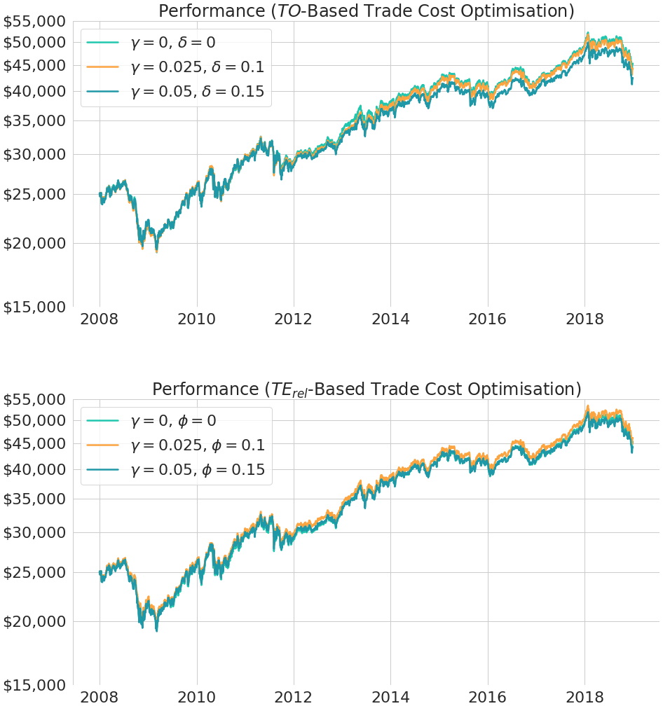
In Figure 1 we present the resulting backtest performance. The first plot corresponds to the -based trade cost optimisation and the second plot to the -based one. We clearly see that the -based trade cost optimisation is capable of producing a performance which is even closer to the ideal strategy performance than for the -based approach. Note that we use a log-scaled y-axis to make it easier to compare relative performance and differences of relative performance over time.
Table 1 summarises the results. We can see that the ex-post relative tracking error can be substantially reduced with the more sophisticated trade cost optimisation approach, attending a minimum of 5.95% for the parameter setting , . At the same time, we also observe that the improved tracking in terms of more similar returns comes at a cost. First, the average daily turnover distances increase, meaning that investors looking at the portfolio weights see larger differences to the target weights than before. However, the dispersion of realised portfolio returns, measured in terms of relative tracking error, becomes smaller. Secondly, the costs of implementation are slightly higher than for the -based trade cost optimisation, but still very low with an average number of 40 and 66 trades per year for the two different parameter settings.
Parameters & metrics |
No trade cost optimisation |
$ |
$ |
$ |
$ |
|---|---|---|---|---|---|
|
|
|
|
||
|
|
|
|||
Ex-post in % |
0.00 |
9.66 |
14.00 |
5.95 |
8.50 |
Average in % |
0.00 |
5.94 |
9.59 |
7.03 |
10.87 |
Annualised turnover |
1.96 |
0.93 |
0.75 |
1.25 |
1.08 |
Annualised trade count |
1422.25 |
40.33 |
23.67 |
66.00 |
39.42 |
It is also worth mentioning that the tuning parameters of both trade cost optimisation approaches allow investors and managers to specify the optimisation according to their individual utility functions. This means that these trade cost optimisations can, for example, be adjusted to reflect individual cost structures and / or preferences with regards to the distance to the target portfolio of investors and portfolio managers.
As in the first article about trade cost optimisations, we now discuss the technical details and mathematical derivations. Readers not interested in those technical details are encouraged to directly jump to the concluding remarks.
Section 4 is organised as follows. We will first translate the tracking-error-based trade cost optimisation into a standard mixed integer quadratic program (MIQP) with linear (in-)equality constraints in Section 4.1. In Section 4.2 we present the cutting plane algorithm, which allows us to solve quadratic programs by iteratively solving linear programs. A main step of the cutting plane algorithm is a Taylor series approximation of a quadratic constraint. This step is explained in detail in Section 4.3.
If we measure the distance to the target portfolio with relative tracking error, we intend to solve the optimisation problem
with .
We can apply the same augmentation technique, as presented in our first blog article about trade cost optimisation, to linearise all constraints. Our optimisation problem is then formulated as a function of the vector and the relations
are enforced via linear equality constraints. We set and note that this constant does not depend on but only on , which is a fixed portfolio and not adapted during the optimisation. Further note, that the relative tracking-error is non-negative, so we can apply the strictly monotonic transformation to our objective function and still obtain the same optimal results. The objective function becomes
i.e., after augmentation the objective function is a quadratic form in and the optimisation problem becomes a mixed integer quadratic program (MIQP). Solvers for such mixed integer quadratic programs (MIQPs) are not necessarily part of standard software packages for numerical optimisation. Therefore, we now discuss the cutting plane algorithm that can be utilised to solve mixed integer quadratic programs (MIQPs) sequentially with solvers for mixed integer linear programs (MILPs).
The basic idea of the cutting plane algorithm, going back to Kelley (1960), is to solve a convex optimisation problem by sequentially solving linear problems and iteratively adding linear constraints which ensure that we finally solve the convex problem1. In our case, this means that we solve a MIQP by sequentially solving several MILPs and iteratively adding linear constraints which ensure that at the end we solve the MIQP.
For simplicity we skip the integer constraints for a moment and illustrate the functioning of the cutting plane algorithm with a standard quadratic program. Quite generally, we want to solve the quadratic program
with linear inequality constraint. In a first step, the cutting plane algorithm transforms the problem, using a slack variable , into
which is a linear program with quadratic constraint. Solvers for linear programs usually come without an implementation of quadratic constraints. The idea of the cutting-plane algorithm now consists of locally approximating the convex constraint (in our case the quadratic constraint ) using a first-order Taylor series expansion. In the following Section 4.3, we provide more details and explain how the Taylor series approximation of the quadratic constraint works. The Taylor series approximation basically results in adding a linear constraint in every iteration. This procedure, i.e., adding another linear constraint and solving the linear program
with an ever growing set of linear constraints ( and are growing in every iteration) is repeated until the slack variable is close enough (e.g., measured by an absolute and relative tolerance) to the true quadratic value .
To better understand the functioning of the cutting plane algorithm, we want to provide a graphical illustration of the cutting plane algorithm for the trivial one-dimensional quadratic problem
Plots for the cases , and , are shown in Figure 2 on the left and right, respectively.
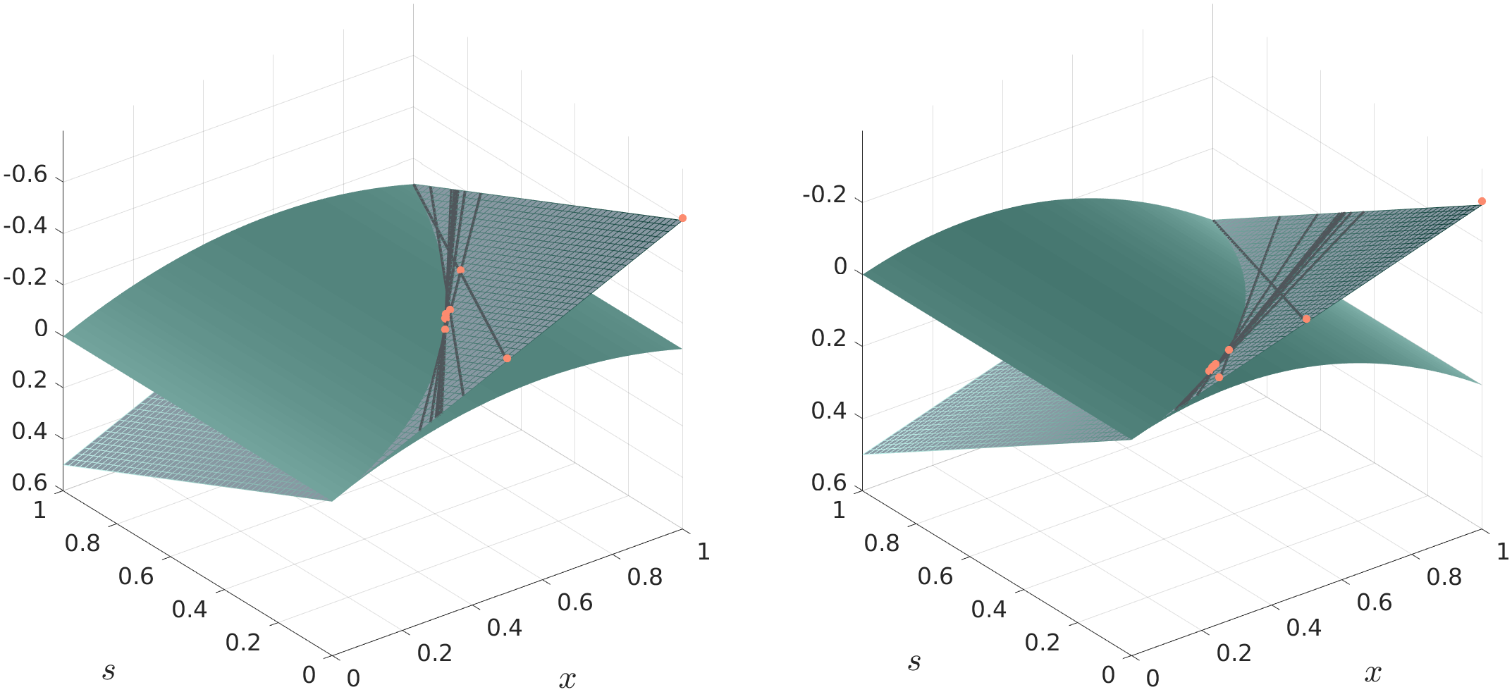
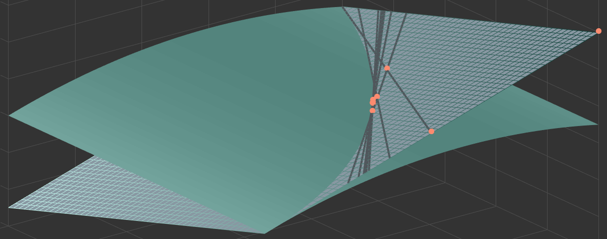
In the three-dimensional plots in Figure 2, the values of the variables and the slack variable are shown on the horizontal axes and the vertical axis represents function values depending on . Note that the plots are flipped upside down. This makes it easier to visualise the iterations of the cutting plane algorithm that is approaching from below (in the flipped plot from above) towards the optimal value at the intersection of the surfaces. Due to the flipped vertical axis the highest values are at the bottom and the lowest values at the top.
Two different surfaces are shown in the plots: The lighter surface is the quadratic objective function of the original optimisation problem
and the darker meshed plane surface represents the linear objective function of the cutting plane optimisation problem
At the intersection of both surfaces, the slack variable is equal to the true quadratic value, i.e., . The cutting plane algorithm now operates on the meshed linear plane. The solution of the optimisation problem is the lowest point on the plane within the linear constraints (represented by grey tangential lines), which force the solver towards the intersection of the two surfaces. This can be nicely seen when looking at the red dots indicating the iterations of the cutting plane algorithm. At the intersection, the slack variable is equal to the true quadratic value and therefore the solution on the linear plane surface is also the solution of the quadratic problem, i.e., the lowest point on the parabolic surface. While the graphical illustration helps to understand the general functioning of the cutting plane algorithm, it is obvious that already in the two-dimensional case, and even more in the general -dimensional case, it is almost impossible to visualise the functioning of the cutting plane algorithm. Nevertheless, we hope that the three-dimensional visualisation of an exemplary one-dimensional problem allows our readers to roughly imagine the functioning in the -dimensional case.
The quadratic constraint is in every iteration linearised by applying a first-order Taylor series expansion. Let , then the first-order Taylor series expansion at is given by
Choose to obtain
Therefore, in each iteration we add the linear inequality constraint
where is just a constant, so we get
For we always use the solution of the optimisation in the previous iteration.
In this blog article, we discussed different measures for the distance of two portfolios. In particular, we provided a comparison of turnover and relative tracking error. We showed why relative tracking error might be deemed superior when measuring the distance to an ideal target portfolio.
Moreover, we developed a tracking-error-based trade cost optimisation and derived an augmented formulation in terms of a classical mixed integer quadratic program (MIQP). To allow a straightforward implementation, we explained how the cutting plane algorithm can be utilised to solve a quadratic program by iteratively solving several linear programs. The benefits of the tracking-error-based trade cost optimisation were shown with backtest results for a momentum portfolio strategy.
Drori, Y. and Teboulle, M. (2016), An optimal variant of Kelley’s cutting-plane method, Mathematical Programming, 160 (1-2), pp. 321-351.
Faber, M. (2010), Relative Strength Strategies for Investing, Available at SSRN: http://dx.doi.org/10.2139/ssrn.1585517.
Kelley, Jr. J. E. (1960), The cutting-plane method for solving convex programs, Journal of the Society for Industrial & Applied Mathematics, 8(4), pp. 703-712.
1: Note that there are several extensions and improved versions of Kelley’s (1960) cutting-plane algorithm (see for example Drori and Teboulle (2016)).
Disclaimer – The views and opinions expressed in this blog are those of the author and do not necessarily reflect the views of Scalable Capital Bank GmbH, its subsidiaries or its employees ("Scalable Capital", "we"). The content is provided to you solely for informational purposes and does not constitute, and should not be construed as, an offer or a solicitation of an offer, advice or recommendation to purchase any securities or other financial instruments. Any representation is for illustrative purposes only and is not representative of any Scalable Capital product or investment strategy. The academic concepts set forth herein are derived from sources believed by the author and Scalable Capital to be reliable and have no connection with the financial services offered by Scalable Capital. Past performance and forward-looking statements are not reliable indicators of future performance. The return may rise or fall as a result of currency fluctuations. Please refer to our risk information.
Risikohinweis – Die Kapitalanlage ist mit Risiken verbunden und kann zum Verlust des eingesetzten Vermögens führen. Weder vergangene Wertentwicklungen noch Prognosen haben eine verlässliche Aussagekraft über zukünftige Wertentwicklungen. Wir erbringen keine Anlage-, Rechts- und/oder Steuerberatung. Sollte diese Website Informationen über den Kapitalmarkt, Finanzinstrumente und/oder sonstige für die Kapitalanlage relevante Themen enthalten, so dienen diese Informationen ausschließlich der allgemeinen Erläuterung der von Unternehmen unserer Unternehmensgruppe erbrachten Wertpapierdienstleistungen. Bitte lesen Sie auch unsere Risikohinweise und Nutzungsbedingungen.