A Python Implementation of Triangles for Visualising Long-Term Investment Metrics

19. Juni 2019 | Dr. Malte Kurz

Disclaimer – The views and opinions expressed in this blog are those of the author and do not necessarily reflect the views of Scalable Capital GmbH or its subsidiaries. Further information can be found at the end of this article.

Summary

We introduce triangle plots for visualising long-term investment metrics.
Return triangles are well suited to showcase the performance of a strategy or asset for a huge number of possible subperiods. Sensitivity analysis with respect to the length of the holding period as well as the start and end dates can thus be easily performed and visualised.
The pairwise comparison of two assets or strategies can be analysed with return triangles for the outperformance in absolute terms or alternatively outperformance indicators can be plotted.
Maximum drawdown and volatility triangles allow to study risks of long-term investments for different subperiods.
The risk and return triangles can be combined to obtain risk-adjusted return triangles.
An open-source python implementation allows readers to generate triangles for their own assets or strategies.

1. Introduction: Triangles for Visualising Long-Term Investment Metrics

With the increased availability of data and computing power, visualisation tools and techniques are becoming more and more important. In an article discussing big data Edd Wilder-James highlighted this when stating:

The art and practice of visualizing data is becoming ever more important in bridging the human-computer gap to mediate analytical insight in a meaningful way.

– Edd Wilder-James in the article "What is big data?" (2012)

Visualisation techniques are a key element when we analyse quantitative investment strategies. In this post we want to open-source and explain one of our tools. The article is equipped with a python implementation to allow our readers to apply the tool for their own analysis. Normally, investors applying quantitative asset allocation techniques have rather long investment horizons. However, the average time of investment of retail investors is maybe between five and fifteen years. Therefore, besides the long-term backtest results asset managers are also interested in analysing subperiods of different lengths. The number of such subperiods is unfortunately increasing rapidly the more data is available and the longer the overall backtest period gets. To do so we propose triangular heatmap plots which allow to visualise a large amount of information in a single plot. Similar triangle plots for visualising long-term investment returns have, for example, been used by The New York Times (2011) and Frankfurter Allgemeine Zeitung (2018). We extend the framework in several regards: First, we provide in Section 6 an open-source implementation for easy generation of the plots. Second, in addition to pure return triangles we also consider triangles for comparing two different strategies or assets with each other in Section 4. Further, we introduce risk triangles, namely maximum drawdown triangles and volatility triangles in Section 5. There, we also propose the natural extension to risk-adjusted return triangles.

2. Prerequisites, Data and the General Functioning of the Triangle Plots

The python implementation presented in Section 6 contains a function called plt_triangle() which is the main interface to obtain the triangle plots. To call plt_triangle(), the user needs to provide a pandas.Series containing discrete percentage returns indexed with dates. If a pd.DataFrame or pd.Series with prices is available such returns can be easily obtained via prices.pct_change() * 100. It is recommended to serve the data series in the highest possible sampling frequency as the target return-frequency can be set via an option. Having provided a return series and a target frequency, the data is down-sampled with pd.Series.resample(). Then returns are aggregated and an annualised return will be computed for every possible subwindow.

For illustrative purposes we will study data from the Kenneth R. French - Data Library (available under: http://mba.tuck.dartmouth.edu/pages/faculty/ken.french/data_library.html) and show examples and code snippets to introduce the functionalities of our triangle tool. In the analysis, we will study factor returns (value, size and momentum) and assume that our hypothetical investor has access to long positions but cannot short sell.¹ Therefore, we compute proxies for the factor returns as $r_{i, t} = frac{1}{2} r_{i, t}^{LS} + r_{Mkt, t}$ , for $i in {Size, Value, Momentum}$ and $r_{i, t}^{LS}$ denotes the original long-short factor return obtained from the data library. The market return is computed as $r_{Mkt} = r_{Mkt-RF} + r_{RF}$ .

Using the python package pandas-datareader, the sample data used in this article can be easily loaded. In the following code, we join the momentum factor to the three classical Fama-French factors and compute the four different factor return series (market, value, size and momentum) used in this article.

import pandas as pd
import numpy as np
import pandas_datareader.data as web

raw_data1 = web.DataReader('F-F_Research_Data_Factors_daily', 'famafrench', start='1900')
raw_data2 = web.DataReader('F-F_Momentum_Factor_daily', 'famafrench', start='1900')

print(raw_data1['DESCR'])
print(raw_data2['DESCR'])

raw_data = raw_data1[0].join(raw_data2[0], how='outer')
raw_data = raw_data.dropna(how='any')
raw_data.columns = raw_data.columns.str.strip()

r_discr_pctg_mkt = raw_data['Mkt-RF'] + raw_data['RF']
r_discr_pctg_val = raw_data['Mkt-RF'] + raw_data['RF'] + 0.5*raw_data['HML']
r_discr_pctg_smb = raw_data['Mkt-RF'] + raw_data['RF'] + 0.5*raw_data['SMB']
r_discr_pctg_mom = raw_data['Mkt-RF'] + raw_data['RF'] + 0.5*raw_data['Mom']

 > F-F Research Data Factors daily
 > -------------------------------
 > 
 > This file was created by CMPT_ME_BEME_RETS_DAILY using the 201903 CRSP
 > database. The T-bill return is the simple daily rate that, over the number of
 > trading days in the month, compounds to 1-month T-Bill rate from Ibbotson and
 > Associates Inc. Copyright 2019 Kenneth R. French
 > 
 >   0 : (24452 rows x 4 cols)
 > F-F Momentum Factor daily
 > -------------------------
 > 
 > This file was created by CMPT_ME_PRIOR_RETS_DAILY using the 201903 CRSP
 > database. It contains a momentum factor, constructed from six value-weight
 > portfolios formed using independent sorts on size and prior return of NYSE,
 > AMEX, and NASDAQ stocks. MOM is the average of the returns on two (big and
 > small) high prior return portfolios minus the average of the returns on two
 > low prior return portfolios. The portfolios are constructed daily. Big means a
 > firm is above the median market cap on the NYSE at the end of the previous day;
 > small firms are below the median NYSE market cap. Prior return is measured from
 > day - 250 to - 21. Firms in the low prior return portfolio are below the 30th
 > NYSE percentile. Those in the high portfolio are above the 70th NYSE
 > percentile. Missing data are indicated by -99.99 or -999.
 > Copyright 2019 Kenneth R. French
 > 
 >   0 : (24351 rows x 1 cols)

3. The Return Triangle

Let us assume that we have a vector of percentage returns ${(r_{t})}_{t=1}^{T}$ and we are interested in a lower frequency. W.l.o.g. there are $N$ disjoint intervals of this lower frequency and $mathcal{I}_n subset {1,ldots,T}$ , for $1leq n leq N$ denotes the index sets for each of these intervals. The percentage return for return interval $n$ can then be obtained as (for $1leq n leq N$ )

R_{n,n} = 100 cdot bigg(prod_{iinmathcal{I}_n} (1 + frac{r_{i}}{100}) - 1bigg)

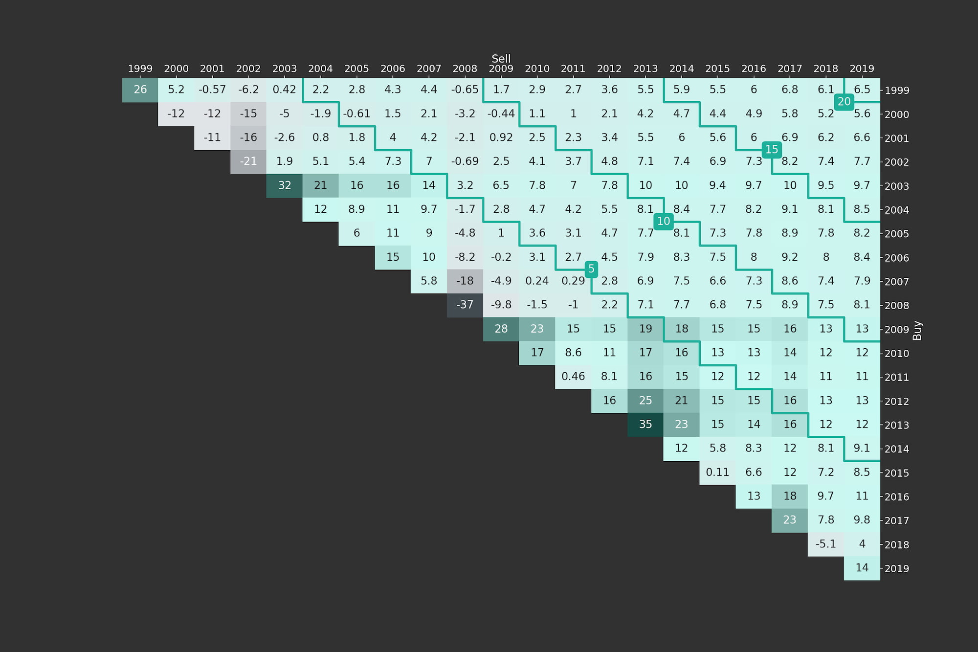
and can be found in the return triangle on the diagonal, i.e, the index ${}_{n,n}$ corresponds to the position in the matrix. To explain the functioning of return triangles, we generated one for the market portfolio between Jan-1999 and Mar-2019, i.e., roughly 20 years of data. We choose a yearly target frequency and the triangle is shown in Figure 1. In the first upper diagonal, the returns correspond to intervals of the length of two periods of the target frequency. Meaning that the entries on the first upper diagonal of the return triangle can be obtained as (for $n=1,ldots,N-1$ )

begin{aligned}R_{n, n+1} &= 100 cdot bigg(Big(prod_{i=0}^{1} (1 + frac{R_{n+i,n+i}}{100})Big)^{frac{1}{2}} - 1bigg) &= 100 cdot bigg(Big(prod_{iin mathcal{I}_{n} cup mathcal{I}_{n+1} } (1 + frac{r_{i}}{100})Big)^{frac{1}{2}} - 1bigg),end{aligned}

where we standardise by applying the square root such that every entry in the triangle is standardised to the length of one interval of the target frequency. In general the entries of the return triangle are defined as (for $j=0,ldots, N-1$ , $n=1,ldots,N-j$ )

R_{n, n+j} = 100 cdot bigg(Big(prod_{i in mathcal{I}_{n, n+j}} (1 + frac{r_{i}}{100})Big)^{frac{1}{j+1}} - 1bigg),

where the index set is given by $mathcal{I}_{n, n+j} := bigcup_{i=0}^{j} mathcal{I}_{n+i}$ . A first example of a return triangle is given in Figure 1. To generate the plot simply copy-paste the code from Section 6 into a .py-file. Choose a module name and use it as file name, e.g., scalable_triangle_utils.py and import the function plt_triangle. To obtain the plot in Figure 1, we call:

from scalable_triangle_utils import plt_triangle

ax = plt_triangle(r_discr_pctg_mkt[r_discr_pctg_mkt.index > '1999'], 'Y');

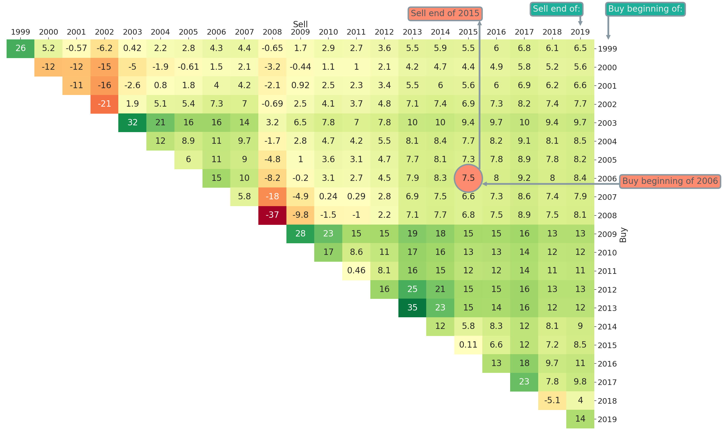
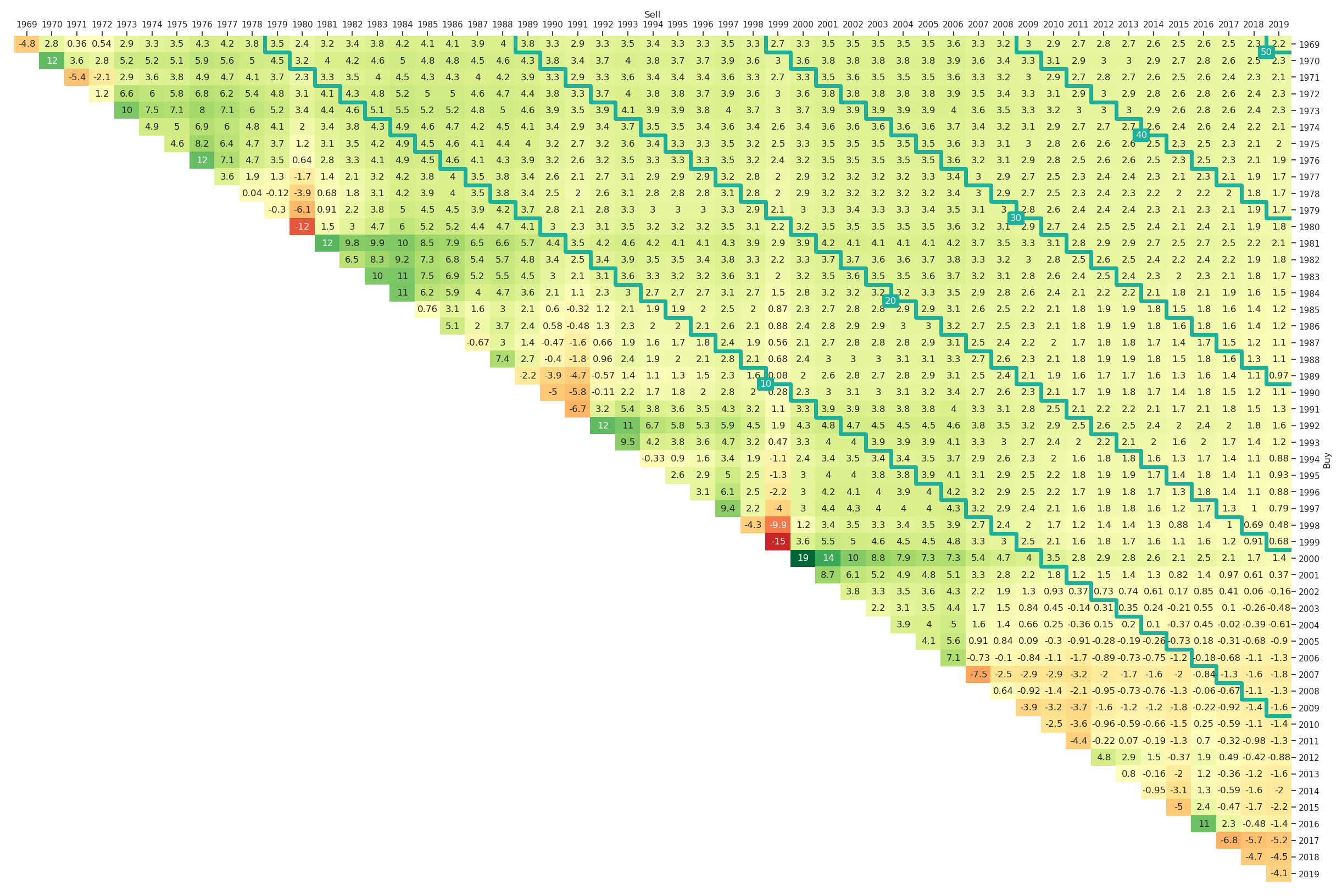
Figure 1: Return (Upper) Triangle for the Fama-French Market Portfolio (yearly, Jan-1999 to Mar-2019)

In Figure 1 we added some annotations to further explain the entries of the triangle plot. The highlighted entry with value 7.5% is the average annual return earned if one invests into the market at the beginning of 2006 and sells after ten years at the end of 2015. In general, the rows represent the year of purchase and the columns the year of selling the asset or strategy being visualised. Therefore, on the main diagonal of Figure 1 all entries correspond to a holding period of one year and on the first upper diagonal all entries correspond to a holding period of two years and so on. This means that by moving to the top right (i.e., further to the right and/or further to the top) the investment horizon is increasing. Naturally, it helps a lot to introduce some diagonal marks for easier orientation. Those marks in the form of stairs can be altered via the optional input mark_periods. For an annual resampling frequency, we could for example mark all holding periods being multiples of five years by setting mark_periods = 5. This is done in Figure 2, where we see stairs annotated with 5, 10, 15 and 20. The highlighted diagonal contains all possible 10-year investment periods within the studied sample period between 1999 and 2019.

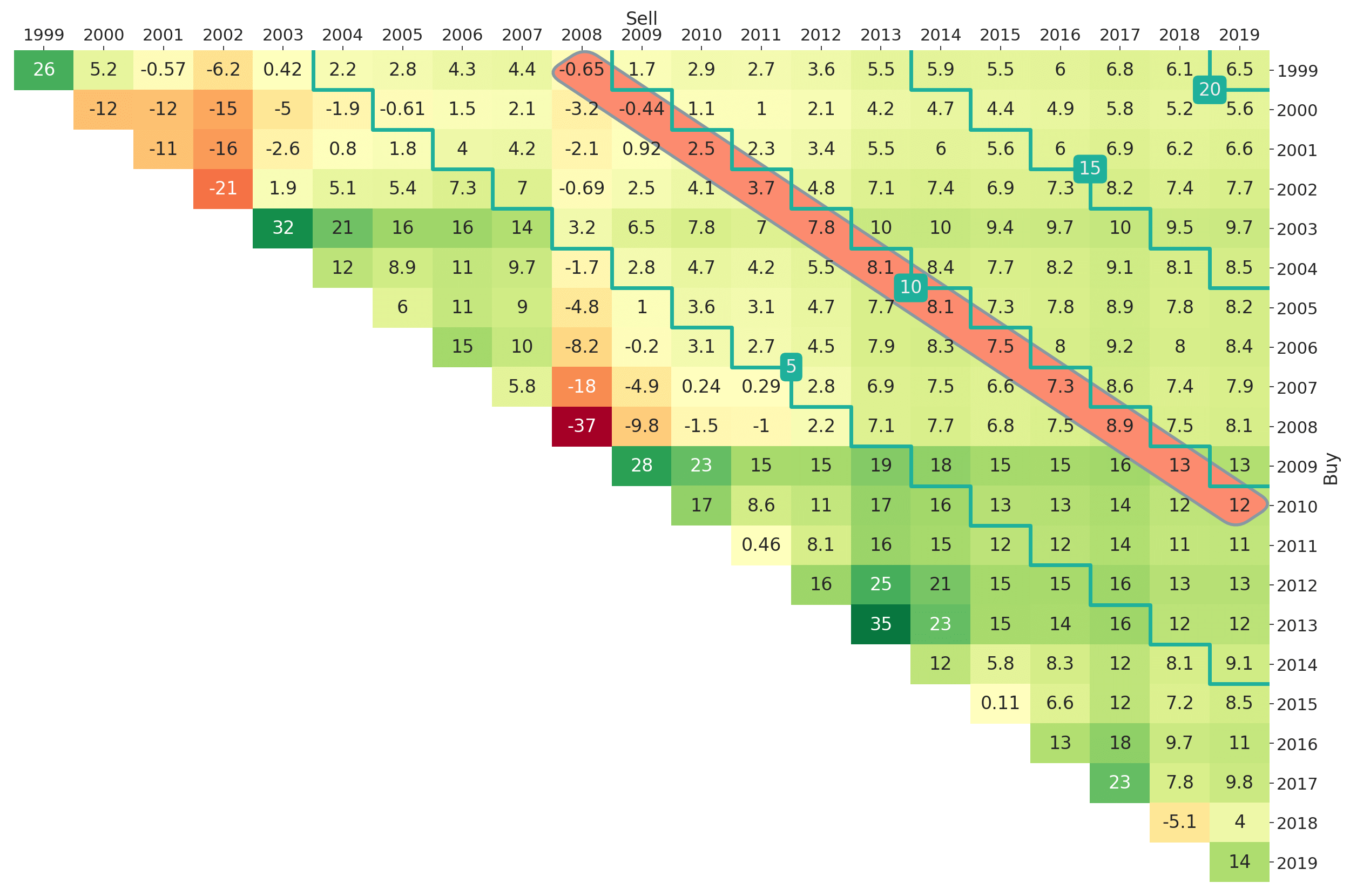
Figure 2: Return Triangle for the Fama-French Market Portfolio (yearly, Jan-1999 to Mar-2019)

The plot in Figure 2 can be obtained via

ax = plt_triangle(r_discr_pctg_mkt[r_discr_pctg_mkt.index > '1999'], 'Y',
                  mark_periods=5);

3.1 Options and Variations of Return Triangles

The function plt_triangle() allows users to customise their return triangle plots. For example via annot = True | False one can determine whether numbers should be shown in cells of the heatmap plot. The variables vmin and vmax can be used to normalise the colourmap. This is particularly useful if return triangles for several competing strategies should be compared directly and one wants to make sure that the colour-coding is aligned. Another option is triangle_type = upper | lower, which can be used to choose between a lower and upper triangle as plot type. As an example, we provide the lower triangle counterpart of Figure 2 in Figure 3. The triangle in Figure 3 can be obtained via

ax = plt_triangle(r_discr_pctg_mkt[r_discr_pctg_mkt.index > '1999'], 'Y',
                  mark_periods=5, triangle_type='lower');

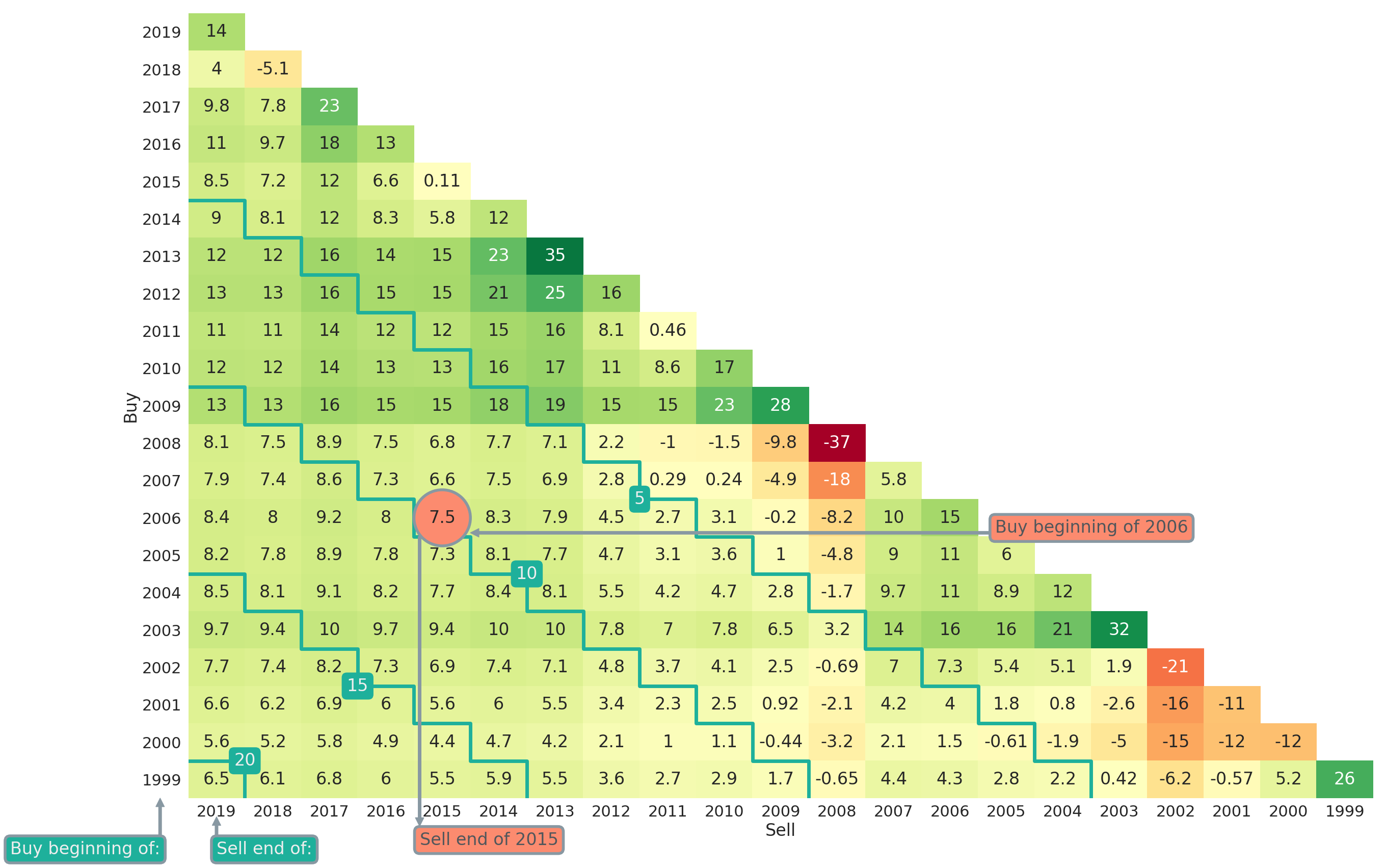
Figure 3: Return (Lower) Triangle for Fama-French Market Portfolio (yearly, Jan-1999 to Mar-2019)

Note that in Figure 3 the investment horizon is now getting larger the more one is moving to the lower left in the triangle plot. All formulas, and especially the indices, in this article will refer to upper triangle plots though.

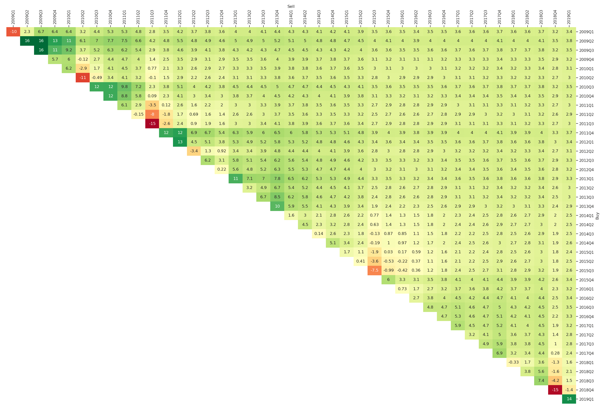
If one is interested in a finer granularity of the overall investment period, one can adapt the resampling rule. For example in Figure 4, we consider quarterly investment periods between 2009 and 2019. The plot can be obtained via

plt_triangle(r_discr_pctg_mkt[r_discr_pctg_mkt.index > '2009'], 'Q');

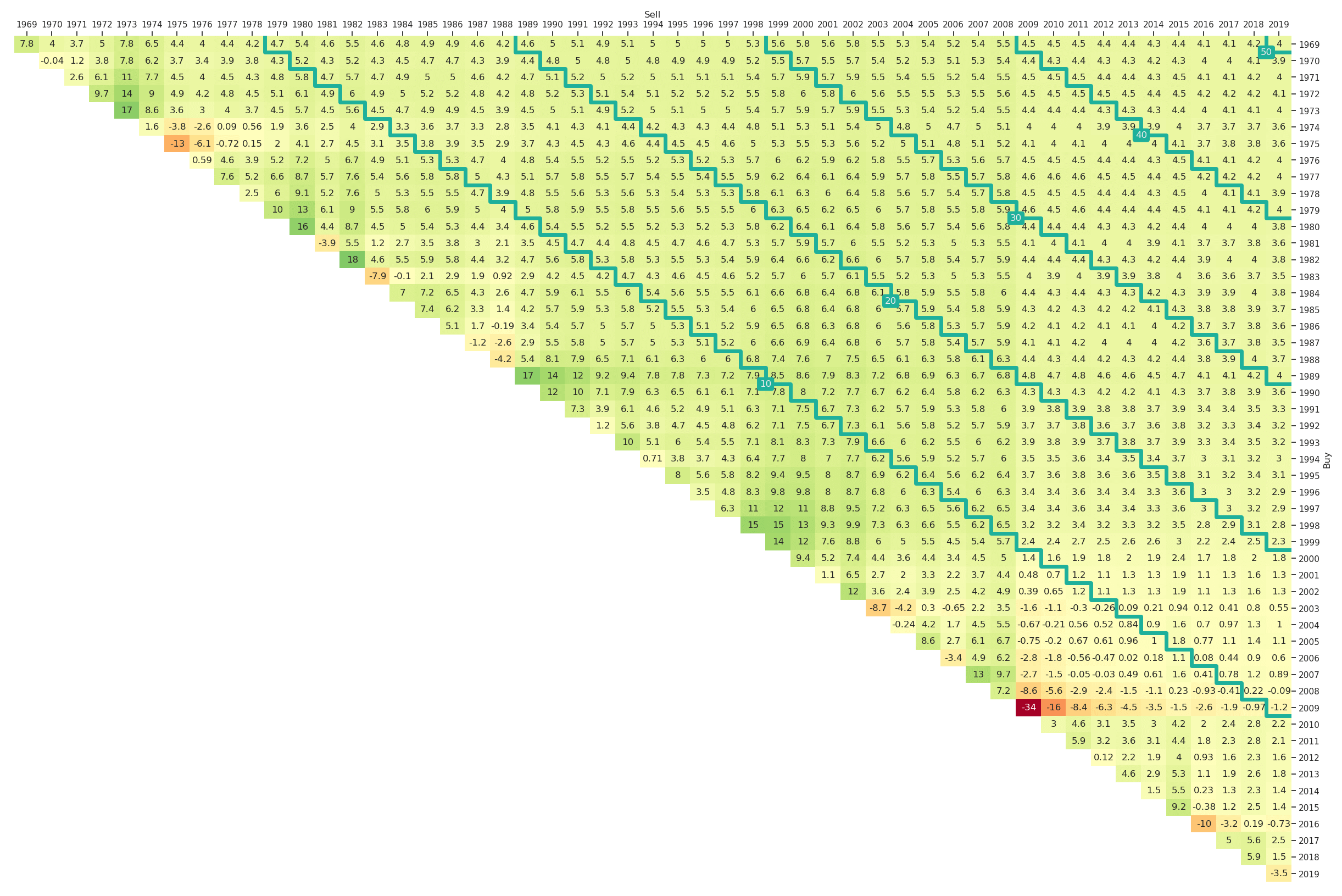
Figure 4: Return Triangle for the Fama-French Market Portfolio (quarterly, Jan-2009 to Mar-2019)

4. Pairwise Comparison of Return Triangles

An important component of many analyses is the comparison against benchmarks. As an example we study long-only investments into the factor portfolios value, size or momentum. Instead of analyzing the absolute performance of these factor portfolios, we benchmark it against an investment into the market portfolio. Two different kinds of visualisation will be shown: The outperformance in absolute terms as well as indicators of outperformance.

4.1 Return Triangles of Outperformance in Absolute Terms

Let us assume that we have computed the entries, $R_{n,n+j}$ , of the return triangle of an asset or strategy of interest and we want to compare it to a benchmark for which we also obtain the return triangle entries $R_{n,n+j}^{B}$ . The outperformance return triangle (in absolute terms) is then defined as

R_{n,n+j}^{Delta, B} = R_{n,n+j} - R_{n,n+j}^{B}.

The corresponding comparative return triangles for value, size and momentum vs. the market are presented in Figure 5, Figure 6 and Figure 7, respectively. The python code to generate them is

ax = plt_triangle(r_discr_pctg_val[r_discr_pctg_val.index > '1969'], 'Y',
                  r_discr_pctg_bench=r_discr_pctg_mkt[r_discr_pctg_mkt.index > '1969'],
                  mark_periods=10);
ax = plt_triangle(r_discr_pctg_smb[r_discr_pctg_smb.index > '1969'], 'Y',
                  r_discr_pctg_bench=r_discr_pctg_mkt[r_discr_pctg_mkt.index > '1969'],
                  mark_periods=10);
ax = plt_triangle(r_discr_pctg_mom[r_discr_pctg_mom.index > '1969'], 'Y',
                  r_discr_pctg_bench=r_discr_pctg_mkt[r_discr_pctg_mkt.index > '1969'],
                  mark_periods=10);

Figure 5: Outperformance of the Long-Only Fama-French Value Factor Portfolio vs. the Market Portfolio (yearly, Jan-1969 to Mar-2019)

Figure 6: Outperformance of the Long-Only Fama-French Size Factor Portfolio vs. the Market Portfolio (yearly, Jan-1969 to Mar-2019)

Figure 7: Outperformance of the Long-Only Fama-French Momentum Factor Portfolio vs. the Market Portfolio (yearly, Jan-1969 to Mar-2019)

4.2 Outperformance Indicator Triangles

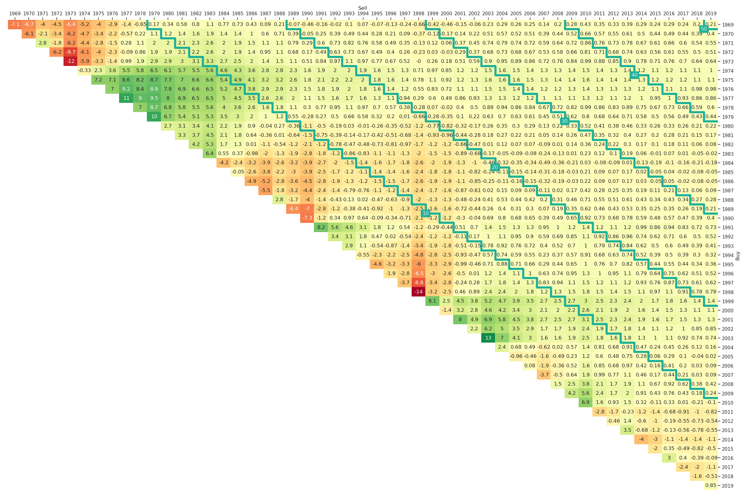
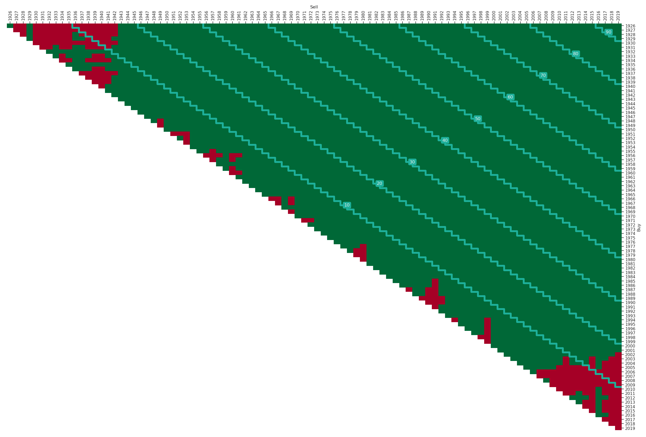
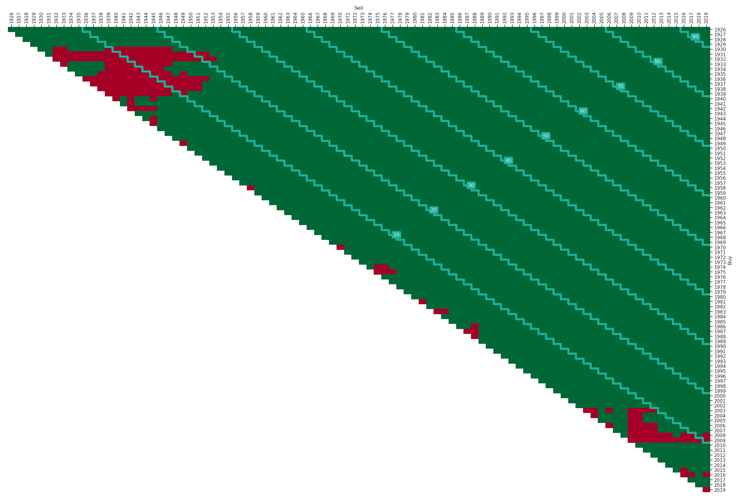
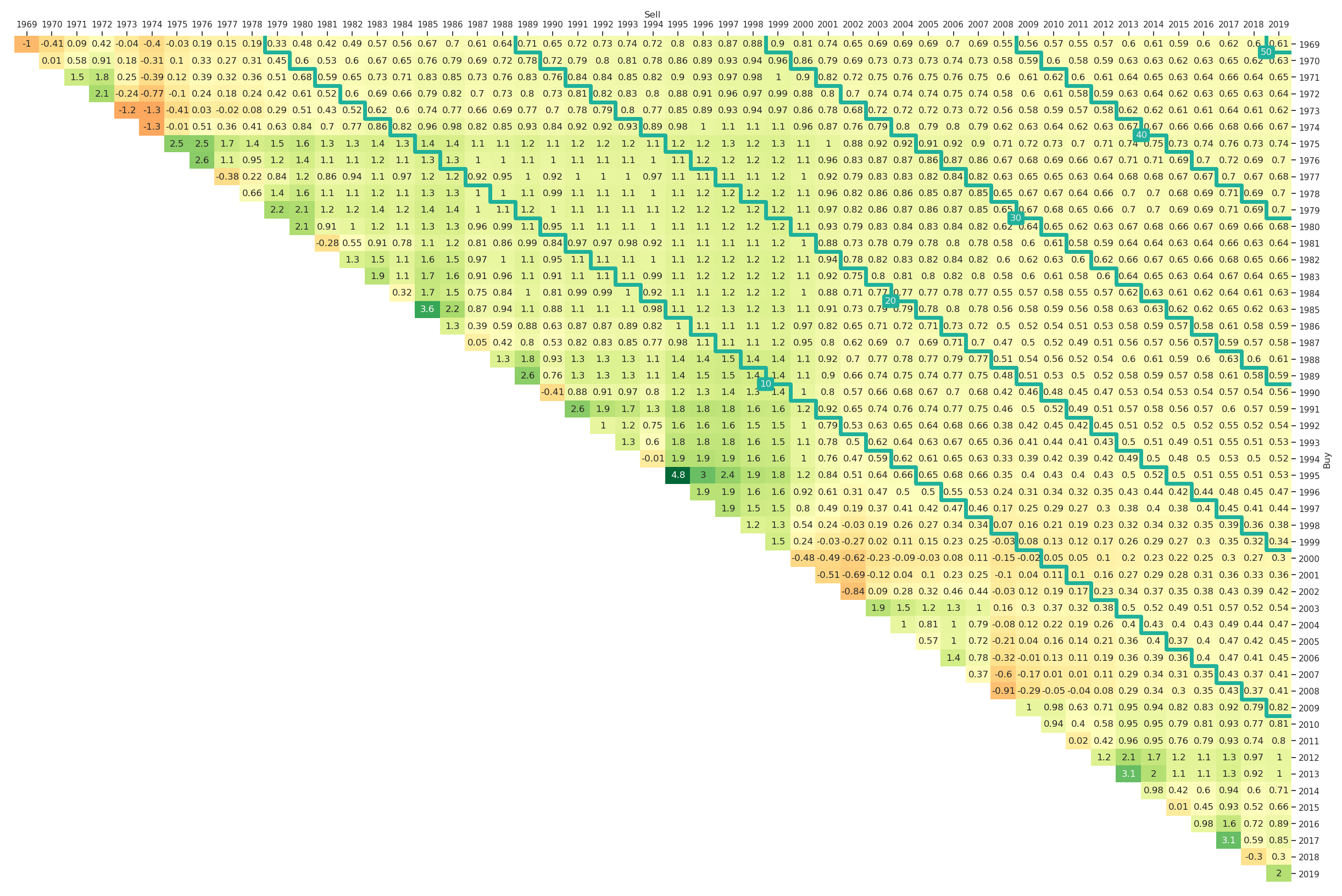
The nice thing about Fama-French factor portfolios is the data availability back to 1926. If we want to analyse such a huge amount of data, the outperformance return triangles become difficult to visualise as they have too many entries. A possible alternative is to focus on indicators instead of deltas, i.e., we are not determining by which amount a strategy outperforms but just whether it outperforms for the corresponding period. The entries in the outperformance indicator triangle are True (green) whenever $R_{n,n+j}^{Delta, B}$ is positive, which is equivalent to $R_{n,n+j} > R_{n,n+j}^{B}$ , and False (red) otherwise. These outperformance indicator return triangles for value, size and momentum vs. the market are shown in Figure 8, Figure 9 and Figure 10, respectively. The corresponding python code is

ax = plt_triangle(r_discr_pctg_val, 'Y',
                  r_discr_pctg_bench=r_discr_pctg_mkt,
                  mark_periods=10, outperf_ind=True);
ax = plt_triangle(r_discr_pctg_smb, 'Y',
                  r_discr_pctg_bench=r_discr_pctg_mkt,
                  mark_periods=10, outperf_ind=True);
ax = plt_triangle(r_discr_pctg_mom, 'Y',
                  r_discr_pctg_bench=r_discr_pctg_mkt,
                  mark_periods=10, outperf_ind=True);

Figure 8, Figure 9 and Figure 10 provide some interesting insights for the long-term performance of factor investing. Again the diagonal stairs are helpful marks for orientation. For example one can see in Figure 8 that the long-only investment into the value factor portfolio outperformed the market portfolio whenever the investment period was longer than 20 years irrespectively of the starting date. For the momentum factor (Figure 10) it is rather similar, with only one area of exception when investing in the beginning of the 1930s. The triangle for the size factor in Figure 9 contains more red underperformance entries with one entry even above the 50-years investment horizon diagonal.

Figure 8: Outperformance Indicators of the Long-Only Fama-French Value Factor Portfolio vs. the Market Portfolio (yearly, Jan-1969 to Mar-2019)

Figure 9: Outperformance Indicators of the Long-Only Fama-French Size Factor Portfolio vs. the Market Portfolio (yearly, Jan-1969 to Mar-2019)

Figure 10: Outperformance Indicators of the Long-Only Fama-French Momentum Factor Portfolio vs. the Market Portfolio (yearly, Jan-1969 to Mar-2019)

5. Risk Triangles

Besides the performance of an investment strategy or asset, a second group of metrics of great relevance for asset managers and retail investors are risk measures. Risk measures, like maximum drawdowns or volatilities can also be easily visualised using triangles to show all possible subperiods of a specific duration. We will introduce two different kinds of risk triangles, the maximum drawdown triangle and the volatility triangle. Additionally, we provide the functionality to generate risk-adjusted return triangles by standardising return triangles with risk triangles.

5.1 The Drawdown Triangle

One possible risk-measure for investment strategies as well as single assets is the maximum drawdown. We obtain cumulative performance series from our return series for the $n$ -th interval as

P_{t, mathcal{I}_n} = prod_{iinmathcal{I}_n, i leq t} (1 + frac{r_{i}}{100}),

for each $t in mathcal{I}_n subset {1, ldots, T}$ . The corresponding maximum drawdown for an interval $mathcal{I}_n$ is now defined as

MDD({mathcal{I}_n}) = 100 cdot bigg( max_{tau in mathcal{I}_n} bigg{frac{P_{tau,mathcal{I}_n}}{max_{tinmathcal{I}_n, tleqtau}{P_{t,mathcal{I}_n} }}bigg} - 1bigg).

The entries of the maximum drawdown triangle are then given by $MDD({mathcal{I}_{n,n+j}})$ , for $j=0,ldots, N-1$ , $n=1,ldots,N-j$ and with the same index sets as for the return triangles given by $mathcal{I}_{n, n+j} := bigcup_{i=0}^{j} mathcal{I}_{n+i}$ .
Note that by construction the monotonicity

MDD({mathcal{I}}) leq MDD({mathcal{J}})

holds whenever $mathcal{I} subseteq mathcal{J}$ irrespectively whether the index set $mathcal{I}$ is consecutively increased at the beginning or the end to obtain the larger set $mathcal{J}$ .

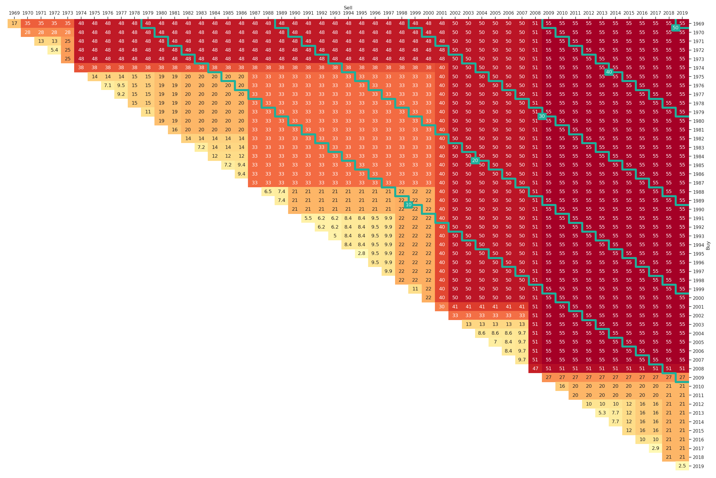
For the market portfolio the maximum drawdown triangle for the past 50 years (1969 to 2019) is shown in Figure 11. It can be easily generated by altering the plt_type, i.e,

ax = plt_triangle(r_discr_pctg_mkt[r_discr_pctg_mkt.index > '1969'], 'Y',
                 plt_type='dd', mark_periods=10,
                 cmap=plt.get_cmap("RdYlGn_r"));

Note that we additionally have chosen a different colourmap 'RdYlGn_r' as higher drawdowns represent higher risks and therefore the reversed version of the default colourmap is more appropriate. In Figure 11 we can for example learn that in the past fifty years the lowest possible maximum drawdown for a ten-year investment horizon was 20% and the highest 55%. The variation of maximum drawdown values by construction tends to be smaller for longer investment horizons. For example for a thirty-year investment in the market an investor would have suffered a maximum drawdown of between 48% and 55% depending on the start date.

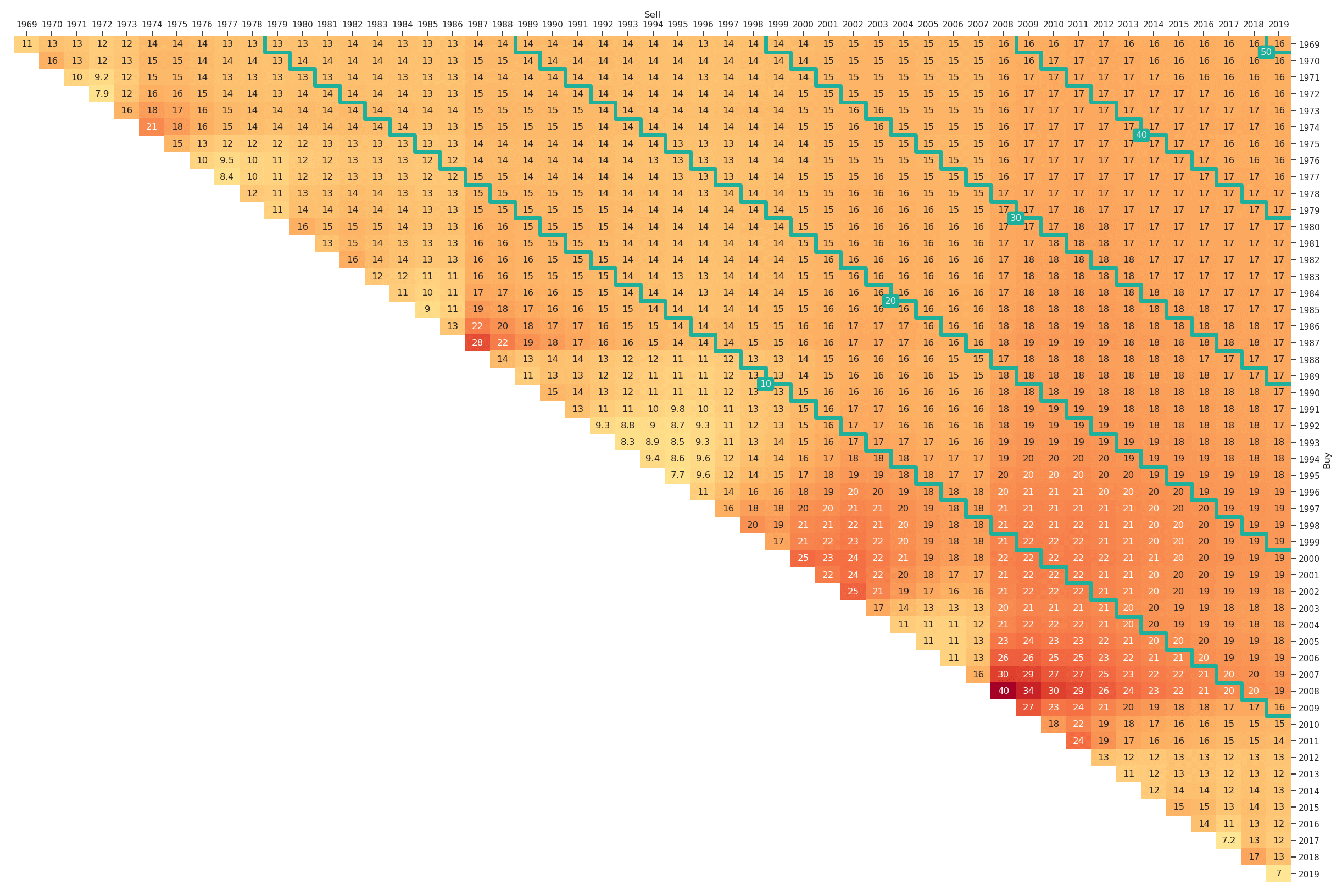
Figure 11: Maximum Drawdown Triangle for the Fama-French Market Portfolio (yearly, Jan-1969 to Mar-2019)

5.2 The Volatility Triangle

As an alternative to the maximum drawdown triangles, we can also consider volatility triangles. In order to obtain entries in a volatility triangle some assumptions need to be made. For simplicity, we estimate sample volatilities using the highest possible return sampling frequency and then apply the square-root-of-time scaling rule to obtain estimates for the period length specified via the resampling rule option. A main reason for relying on this assumption is that we also want to be able to provide somewhat reliable estimates on the main and first diagonals. This would not be possible when first aggregating returns, as we would then have to estimate volatilities from a single, or a small number of observations. Nevertheless, when interpreting the volatility triangles one should be aware that they rely on some assumptions like square-root-of-time scaling.

The entries of the volatility triangle are defined as (for $j=0,ldots, N-1$ , $n=1,ldots,N-j$ )

sigma_{n, n+j} = bigg(frac{#(mathcal{I}_{n, n+j})}{j+1} Big(frac{1}{#(mathcal{I}_{n, n+j}) - 1} sum_{i in mathcal{I}_{n, n+j}} (r_{i} - bar{r})^2 Big) bigg)^{frac{1}{2}},

where the index set is given by $mathcal{I}_{n, n+j} := bigcup_{i=0}^{j} mathcal{I}_{n+i}$ . Additionally, $bar{r}$ denotes the sample mean $bar{r} = frac{1}{#(mathcal{I}_{n, n+j})} sum_{i in mathcal{I}_{n, n+j}} r_{i}$ and $#(mathcal{I}_{n, n+j})$ the cardinality of the index set $mathcal{I}_{n, n+j}$ .

Also the volatility triangle can be easily generated by altering the plt_type and is shown in Figure 12.

ax = plt_triangle(r_discr_pctg_mkt[r_discr_pctg_mkt.index > '1969'], 'Y',
                 plt_type='vol', mark_periods=10,
                 cmap=plt.get_cmap("RdYlGn_r"));

Figure 12: Volatility Triangle for the Fama-French Market Portfolio (yearly, Jan-1969 to Mar-2019)

5.3 The Risk-Adjusted Return Triangles

A natural extension to the risk and return triangles are risk-adjusted return triangles. Our implementation allows for adjusting returns with respect to either volatility or maximum drawdowns. As a result, one obtains Sharpe ratios (one might want to use excess returns as input to the return triangle function) and return-drawdown ratios. To illustrate the interface, we provide the risk-adjusted (with respect to volatility) return triangle for the market portfolio in Figure 13. The interface can be called via

ax = plt_triangle(r_discr_pctg_mkt[r_discr_pctg_mkt.index > '1969'], 'Y',
                 mark_periods=10, risk_adjusted='vol');

Figure 13: Risk-Adjusted Return Triangle for the Fama-French Market Portfolio (yearly, Jan-1969 to Mar-2019)

6. An Implementation in Python

This sections contains a python implementation for all presented triangles. The main function is plt_triangle(). The first two input variables r_discr_pctg (a pandas.Series containing discrete percentage returns indexed with dates) and resampling_rule (the target frequency) are mandatory. All other inputs are optional and can be used to customise your triangle plot.

To get started choose a module name and use it as file name, e.g., scalable_triangle_utils.py and import the function plt_triangle. Besides the main function delivering the triangle plots, three functions for the actual computations are defined. The functions compute_ret_triangle(), compute_dd_triangle() and compute_vol_triangle() can be used to obtain the entries of return, maximum drawdown and volatility triangles, respectively. The module relies on some dependencies, mainly the pandas package and the heatmap plot from the seaborn package.

#### LICENSE ####
# MIT License

# Copyright (c) 2019 Scalable Capital GmbH

# Permission is hereby granted, free of charge, to any person obtaining a copy
# of this software and associated documentation files (the "Software"), to deal
# in the Software without restriction, including without limitation the rights
# to use, copy, modify, merge, publish, distribute, sublicense, and/or sell
# copies of the Software, and to permit persons to whom the Software is
# furnished to do so, subject to the following conditions:

# The above copyright notice and this permission notice shall be included in all
# copies or substantial portions of the Software.

# THE SOFTWARE IS PROVIDED "AS IS", WITHOUT WARRANTY OF ANY KIND, EXPRESS OR
# IMPLIED, INCLUDING BUT NOT LIMITED TO THE WARRANTIES OF MERCHANTABILITY,
# FITNESS FOR A PARTICULAR PURPOSE AND NONINFRINGEMENT. IN NO EVENT SHALL THE
# AUTHORS OR COPYRIGHT HOLDERS BE LIABLE FOR ANY CLAIM, DAMAGES OR OTHER
# LIABILITY, WHETHER IN AN ACTION OF CONTRACT, TORT OR OTHERWISE, ARISING FROM,
# OUT OF OR IN CONNECTION WITH THE SOFTWARE OR THE USE OR OTHER DEALINGS IN THE
# SOFTWARE.
#### LICENSE ####

import pandas as pd
import numpy as np
from scipy import stats

import matplotlib.pyplot as plt
import seaborn as sns

def plt_triangle(r_discr_pctg, resampling_rule, plt_type = 'ret', r_discr_pctg_bench=None,
                 mark_periods=None, annot=True, outperf_ind=False, risk_adjusted = None,
                 cmap=plt.get_cmap("RdYlGn"), mark_period_linewidth=5, vmin=None, vmax=None,
                 triangle_type='upper'):
    assert isinstance(r_discr_pctg, pd.Series)
    assert triangle_type in ['lower', 'upper']

    r_discr_resampled = resample_r_discr_pctg(r_discr_pctg, resampling_rule)

    n_periods = len(r_discr_resampled)

    if plt_type == 'ret':
        df_r_triangle = compute_ret_triangle(r_discr_resampled, triangle_type)
        if risk_adjusted is not None:
            if risk_adjusted == 'dd':
                df_risk = compute_dd_triangle(r_discr_pctg, r_discr_resampled.index, triangle_type)
            elif risk_adjusted == 'vol':
                df_risk = compute_vol_triangle(r_discr_pctg, r_discr_resampled.index, triangle_type)
            else:
                raise ValueError('Invalid risk_adjusted')
            df_r_triangle = df_r_triangle.divide(df_risk)
    else:
        assert risk_adjusted is None
        if plt_type == 'dd':
            df_r_triangle = compute_dd_triangle(r_discr_pctg, r_discr_resampled.index, triangle_type)
        elif plt_type == 'vol':
            df_r_triangle = compute_vol_triangle(r_discr_pctg, r_discr_resampled.index, triangle_type)
        else:
            raise ValueError('Invalid plt_type')

    if isinstance(r_discr_pctg_bench, pd.Series):
        pd.testing.assert_index_equal(r_discr_pctg.index, r_discr_pctg_bench.index)
        r_discr_bench_resampled = resample_r_discr_pctg(r_discr_pctg_bench, resampling_rule)
        df_r_triangle_bench = compute_ret_triangle(r_discr_bench_resampled, triangle_type)
        df_r_triangle = df_r_triangle - df_r_triangle_bench
    else:
        assert r_discr_pctg_bench is None, 'provide pd.Series as benchmark'

    if outperf_ind:
        plt_data = df_r_triangle.copy()>0
        plt_data = plt_data.astype(float)
        plt_data[df_r_triangle.isna()] = np.nan
        annot = False
    else:
        plt_data = df_r_triangle.round(2)

    r_triangle_ax = sns.heatmap(plt_data,
                                cmap=cmap, cbar=False,
                                center=0.5, annot=annot, linewidths=0,
                                vmin=vmin, vmax=vmax)
    r_triangle_ax.set_facecolor('None')

    plt.xlabel('Sell')
    plt.ylabel('Buy')
    if triangle_type == 'upper':
        rot = r_triangle_ax.get_xticklabels()[0].get_rotation()
        r_triangle_ax.xaxis.set_ticks_position('top')
        plt.xticks(rotation=rot)

        rot = r_triangle_ax.get_yticklabels()[0].get_rotation()
        r_triangle_ax.yaxis.set_ticks_position('right')
        plt.yticks(rotation=rot)

        r_triangle_ax.xaxis.set_label_position('top')
        r_triangle_ax.yaxis.set_label_position('right')

    if mark_periods is not None:
        marker_positions = np.arange(int(mark_periods), n_periods, int(mark_periods))
        for this_mark_period in marker_positions:
            x_vals = np.arange(0,n_periods+1-this_mark_period,1)
            y_vals = np.arange(this_mark_period,n_periods+1,1)
            if triangle_type == 'upper':
                x_vals, y_vals = y_vals, x_vals
                where = 'pre'
            else:
                where = 'post'
            r_triangle_ax.step(x_vals, y_vals, linewidth = mark_period_linewidth,
                               color='#1EB09B', where=where);

            x_pos = x_vals[int(np.floor(len(x_vals)/2))]
            y_pos = y_vals[int(np.floor(len(y_vals)/2))]
            if len(x_vals) % 2 == 0:
                if triangle_type == 'lower':
                    y_pos = y_vals[int(np.floor(len(y_vals)/2)) - 1]
                else:
                    x_pos = x_vals[int(np.floor(len(x_vals)/2)) - 1]

            plt.text(x=x_pos, y=y_pos, s=str(this_mark_period), color = '#EEEEEE',
                     bbox=dict(boxstyle='round', facecolor='#1EB09B', edgecolor='none'),
                     ha='center', va='center')

    return r_triangle_ax

def compute_ret_triangle(r_discr_pctg, triangle_type):
    n_periods = len(r_discr_pctg)

    r_triangle = np.full([n_periods, n_periods], np.nan)
    for i_period in range(0, n_periods):
        for j_period in range(i_period, n_periods):
            r_triangle[i_period, j_period] = (stats.gmean(1 + r_discr_pctg.iloc[i_period:j_period+1]/100) - 1)*100

    df_r_triangle = pd.DataFrame(r_triangle,
                                 index=r_discr_pctg.index,
                                 columns=r_discr_pctg.index)

    if triangle_type == 'lower':
        df_r_triangle.sort_index(0, ascending=False, inplace=True)
        df_r_triangle.sort_index(1, ascending=False, inplace=True)

    return df_r_triangle

def resample_r_discr_pctg(r_discr_pctg, resampling_rule):
    r_discr_resampled = (((1+r_discr_pctg/100).resample(resampling_rule).prod()-1)*100)
    r_discr_resampled.index = r_discr_resampled.index.to_period(resampling_rule)

    return r_discr_resampled

def max_ddown(price_time_series):
    cum_max_prices = price_time_series.cummax()
    ddowns = 100 * (price_time_series / cum_max_prices - 1)

    ddowns_no_nan = ddowns.dropna()
    max_dd = abs(min(ddowns_no_nan))

    return max_dd

def extract_sub_window(s, f, t):
    ind = np.logical_and((s.index > f),
                         (s.index <= t))
    return s[ind]

def compute_dd_triangle(r_discr_pctg, period_ind, triangle_type):
    n_periods = len(period_ind)
    time_thres = period_ind[0:1].to_timestamp(how='S').append(period_ind.to_timestamp(how='E'))

    dd_triangle = np.full([n_periods, n_periods], np.nan)
    for i_period in range(0, n_periods):
        for j_period in range(i_period, n_periods):
            rets = extract_sub_window(r_discr_pctg, time_thres[i_period], time_thres[j_period + 1])
            perfs = (1 + rets/100).cumprod()
            dd_triangle[i_period, j_period] = max_ddown(perfs)

    dd_triangle = pd.DataFrame(dd_triangle,
                               index=period_ind,
                               columns=period_ind)

    if triangle_type == 'lower':
        dd_triangle.sort_index(0, ascending=False, inplace=True)
        dd_triangle.sort_index(1, ascending=False, inplace=True)

    return dd_triangle

def compute_vol_triangle(r_discr_pctg, period_ind, triangle_type):
    n_periods = len(period_ind)
    time_thres = period_ind[0:1].to_timestamp(how='S').append(period_ind.to_timestamp(how='E'))

    vol_triangle = np.full([n_periods, n_periods], np.nan)
    for i_period in range(0, n_periods):
        for j_period in range(i_period, n_periods):
            rets = extract_sub_window(r_discr_pctg, time_thres[i_period], time_thres[j_period + 1])
            n = j_period + 1 - i_period
            vol_triangle[i_period, j_period] = np.sqrt(rets.var() * len(rets)/n)

    vol_triangle = pd.DataFrame(vol_triangle,
                                index = period_ind,
                                columns = period_ind)

    if triangle_type == 'lower':
        vol_triangle.sort_index(0, ascending=False, inplace=True)
        vol_triangle.sort_index(1, ascending=False, inplace=True)

    return vol_triangle

7. Concluding Remarks

In this blog article we introduced triangle plots for visualising long-term investment metrics. To introduce, explain and showcase the general functioning of our triangles we study Fama-French factor data. Return triangles can be used to visualise the performance of strategies or assets for different holding periods and varying start and end dates. In addition, return triangles can also be used to perform pairwise comparisons of different strategies or assets. To study risk measures for different investment horizons we introduced maximum drawdown and volatility triangles. The combination of return and risk triangles gives rise to risk-adjusted return triangles for analysing long-term investment decisions. An open-source python implementation is provided in order to allow readers to generate triangle plots for their own assets or investment strategies.

References

Frankfurter Allgemeine Zeitung (2018), Daniel Mohr, Kaum Verluste mit deutschen Aktien möglich, https://www.faz.net/-iju-95jsr.

The New York Times (2011), In Investing, It’s When You Start And When You Finish, http://archive.nytimes.com/www.nytimes.com/interactive/2011/01/02/business/20110102-metrics-graphic.html#

Wilder-James, E. (2012), What is big data?, https://www.oreilly.com/ideas/what-is-big-data.

1: Note that we use the factor return series as provided in the Kenneth R. French - Data Library. When implementing factor strategies additional trading costs could arise and a direct investment into the factor portfolios might not be possible.

Disclaimer – The views and opinions expressed in this blog are those of the author and do not necessarily reflect the views of Scalable Capital GmbH, its subsidiaries or its employees ("Scalable Capital", "we"). The content is provided to you solely for informational purposes and does not constitute, and should not be construed as, an offer or a solicitation of an offer, advice or recommendation to purchase any securities or other financial instruments. Any representation is for illustrative purposes only and is not representative of any Scalable Capital product or investment strategy. The academic concepts set forth herein are derived from sources believed by the author and Scalable Capital to be reliable and have no connection with the financial services offered by Scalable Capital. Past performance and forward-looking statements are not reliable indicators of future performance. The return may rise or fall as a result of currency fluctuations. Please refer to our risk information.

Risikohinweis – Die Kapitalanlage ist mit Risiken verbunden und kann zum Verlust des eingesetzten Vermögens führen. Weder vergangene Wertentwicklungen noch Prognosen haben eine verlässliche Aussagekraft über zukünftige Wertentwicklungen. Wir erbringen keine Anlage-, Rechts- und/oder Steuerberatung. Sollte diese Website Informationen über den Kapitalmarkt, Finanzinstrumente und/oder sonstige für die Kapitalanlage relevante Themen enthalten, so dienen diese Informationen ausschließlich der allgemeinen Erläuterung der von Unternehmen unserer Unternehmensgruppe erbrachten Wertpapierdienstleistungen. Bitte lesen Sie auch unsere Risikohinweise und Nutzungsbedingungen.

Dr. Malte Kurz

QUANTITATIVE STRATEGIST

Malte works as Quantitative Researcher at Scalable Capital and is a Research Fellow of the Center for Quantitative Risk Analysis at the Ludwig-Maximilians-Universität (LMU) Munich. He studied Mathematical Finance at the University of Konstanz and Statistics at the LMU. He previously worked as a research and teaching assistant at the Chair of Financial Econometrics (LMU). In his PhD thesis he developed and analyzed methods for high-dimensional dependence modelling with applications in financial econometrics. Malte has published peer-reviewed research articles and regularly serves as a referee for academic journals.

Die Kapitalanlage ist mit Risiken verbunden. Der Wert Ihrer Kapitalanlage kann fallen oder steigen. Es kann zu Verlusten des eingesetzten Kapitals kommen. Frühere Wertentwicklungen, Simulationen oder Prognosen sind kein verlässlicher Indikator für die künftige Wertentwicklung. Bitte beachten Sie hierzu unsere Risikohinweise.

Für Neukunden: 4 % p.a. Zinsen (Baader Bank) bis 1 Mio. € für 4 Monate. Danach 2,6 % p.a. variabler Zins bis 100.000 €. Zinsangebot nur mit PRIME+. Mehr Informationen.

Folgen Sie uns

Newsletter abonnieren

Scalable Capital GmbH
Seitzstraße 8e, 80538 München | Kontakt | Impressum
Zuständige Aufsicht: BaFin, Deutsche Bundesbank